the Creative Commons Attribution 4.0 License.
the Creative Commons Attribution 4.0 License.
 | 23 Jan 2020
Impact of local gravity wave forcing in the lower stratosphere on the polar vortex stability: effect of longitudinal displacement
Nadja Samtleben
Aleš Kuchař
Petr Šácha
Petr Pišoft
Christoph Jacobi
The effects of gravity wave (GW) breaking hotspots in the lower stratosphere, especially the role of their longitudinal distribution, are evaluated through a sensitivity study by using a simplified middle atmosphere circulation model. For the position of the local GW hotspot, we first selected a fixed latitude range between 37.5 and 62.5∘ N and a longitude range from 112.5 to 168.75∘ E, as well as an altitude range between 18 and 30 km. This confined GW hotspot was then shifted in longitude by 45∘ steps, so that we created eight artificial GW hotspots in total. Strongly dependent on the location of the respective GW hotspot with regard to the phase of the stationary planetary wave of wavenumber 1 (SPW 1) generated in the model, the local GW forcing may interfere constructively or destructively with the modeled SPW 1. GW hotspots, which are located in North America near the Rocky Mountains, lead to an increase in the SPW 1 amplitude and EP flux, while hotspots located near the Caucasus, the Himalayas or the Scandinavian region lead to a decrease in these parameters. Thus, the polar vortex is less (Caucasus and Himalayan hotspots) or more weakened (Rocky Mountains hotspot) by the prevailing SPW activity. Because the local GW forcing generally suppresses wave propagation at midlatitudes, the SPWs 1 propagate into the polar region, where the refractive index turned to positive values for the majority of the artificial GW hotspots. An additional source of SPW 1 may be local instabilities indicated by the reversal in the meridional potential vorticity gradient in the polar region in connection with a positive EP divergence. In most cases, the SPWs 1 are breaking in the polar region and maintain the deceleration and, thus, the weakening of the polar vortex. While the SPWs 1 that form when the GW hotspots are located above North America propagate through the polar region into the middle atmosphere, the SPWs 1 in the remaining GW hotspot simulations were not able to propagate further upwards because of a negative refractive index above the positive refractive index anomaly in the polar region. GW hotspots, which are located near the Himalayas, influence the mesosphere–lower thermosphere region because of possible local instabilities in the lower mesosphere generating additional SPWs 1, which propagate upwards into the mesosphere.


Atmospheric dynamics is characterized by waves with different spatial and temporal scales (Douville, 2009) mainly forced in the lower part of the atmosphere, i.e., in the troposphere and stratosphere. One of the most important wave types, besides the planetary waves (PWs) and atmospheric tides, are gravity waves (GWs), which maintain the circulation and the thermal structure of the upper atmosphere by exchanging energy and momentum and contributing to turbulence and mixing between all vertical layers (Fritts and Alexander, 2003). Their interaction with PWs (e.g., Manson et al., 2003; Jacobi et al., 2006; Hoffmann et al., 2012) or tides (e.g., Preusse et al., 2001; Beldon and Mitchell, 2010; Senf and Achatz, 2011) can generate secondary waves, which may even influence the thermosphere (Miyahara and Forbes, 1991; Lilienthal et al., 2018). Thus, GWs are one of the main contributors to the coupling of different atmospheric layers. GWs are mainly generated by orography (Smith, 1985; Nastrom and Fritts, 1992), convection (Tsuda et al., 1994), jet sources (Plougonven and Zhang, 2014) or spontaneous adjustment processes (Fritts and Alexander, 2003), but not all of them are able to propagate into the middle atmosphere, which is strongly dependent on their phase speed.
GWs exhibit a large spatial and temporal variability, which is closely linked to the synoptic conditions, the propagation conditions and the source of the GWs. Thus, there is a huge variability in the global GW distribution (Ern et al., 2004; Fröhlich et al., 2007; Hoffmann et al., 2013; Schmidt et al., 2016). Most of the regions of enhanced GW activity are connected to (i) orography (Hoffmann et al., 2013), which is quite stable and persistent in space and time, or (ii) deep convection (in the Tropics; Ern and Preusse, 2012) as well as to jet sources (mainly in the midlatitudes; Plougonven and Zhang, 2014), which are spatially and temporally variable. The phase speed of nonorographically generated GWs (induced by convection, jet sources) differs from the one of orographic GWs, which is highly influencing their propagation into the middle atmosphere (Andrews et al., 1987). Depending on the position, strength and the induced wind shear of, for example, the subtropical and polar front jet (jet sources), the generated GWs are either able to propagate into the mesosphere or break in the lower stratosphere (LS) (Gisinger et al., 2017). Apart from the phase speed the amplitude of all kinds of GWs is also particularly important for the breaking conditions. Upward-propagating GWs having large amplitudes, which increase the instability of the GWs, can already break in the LS (Fritts et al., 2016). These locally breaking GWs in the LS, which occur only sporadically, were already observed by Hoffmann et al. (2013), Šácha et al. (2015) and Fritts et al. (2016). In any case, this leads to a transfer of momentum and energy, also called GW drag, on the local background flow in the LS and may also influence the stability of the polar vortex. In connection with an intensified PW activity, this process can produce a preconditioning of the polar vortex (Šácha et al., 2016; Samtleben et al., 2019) or even a sudden stratospheric warming (SSW) (Albers and Birner, 2014). Such an effect of breaking GWs in the LS has been also observed in several model studies (e.g., Plougonven et al., 2008; Constantino et al., 2015) as well as in satellite measurements showing enhanced GW drag in the stratosphere before SSW events (Ern et al., 2016). Therefore, enhanced GW forcing in the LS may play an important role as a precursor and as an indicator of a potentially arising SSW.
Model experiments already showed that changes in GW parameters, e.g., the GW drag or the momentum flux, which modify the polar vortex geometry or even the stability (Samtleben et al., 2019), can lead to different kinds of vortex breakdowns (splitting or displacement) in connection with PW activity (Šácha et al., 2016; Scheffler et al., 2018). As a result, the vortex geometry, including a weakening or strengthening of the vortex itself, strongly depends on the temporal and spatial GW drag distribution (Scheffler et al., 2018; Samtleben et al., 2019). These approaches provide a new basis regarding the evaluation of SSW events, which are strongly affected by GWs as well as by PWs. In an earlier study (Samtleben et al., 2019) we analyzed the effect of an artificial GW hotspot on the polar vortex. The position was initially East Asia (EA), based on the results of Šácha et al. (2015), and was shifted in latitude. To now provide information about more realistic distributions of GW hotspots, in this study we will displace the EA hotspot in longitude.
Thereby, we capture known GW hotspots like the Himalayas, the Rocky Mountains and several mountains in Europe. Furthermore, the displacement of the GW hotspot is along the polar front jet, so that also nonorographical GWs are considered. However, the chosen GW forcing of each artificial GW hotspot, which is the same for all GW hotspots in our sensitivity study (see Sect. 2.2 or Samtleben et al., 2019), may not represent the corresponding realistic GW hotspot forcing. In reality, the GW forcing strongly depends on the background conditions in the region of the respective GW hotspot, which is influenced by the prevailing stationary planetary wave (SPW) activity. Thus, the realistic GW forcing of each artificial GW hotspot would differ in strength as well as in direction, but this would complicate the interpretation of the results. For this purpose, our sensitivity study is more idealized and simplified. In the following Sect. 2 of this paper, we will briefly describe the global circulation model (GCM) used and will provide details on how the GW hotspots are implemented in this GCM. Section 3 describes and discusses the modeled dynamical effects of the GW hotspots on the circulation of the middle atmosphere, which includes the analysis of SPW activity and the wave propagation conditions. Section 4 concludes the paper.
2.1 Model description and experiments
To analyze the middle atmosphere response to different local GW hotspots in the LS, we performed several experiments using the Middle and Upper Atmosphere Model (MUAM; Pogoreltsev et al., 2007; Lilienthal et al., 2017; Samtleben et al., 2019). MUAM is a mechanistic, 3-D, nonlinear global circulation model, which extends in 56 layers up to an altitude of about 160 km in logarithmic pressure height z with a vertical resolution Δz=2.842 km. The logarithmic pressure height z is defined by with a constant scale height H=7 km and the reference pressure level p0=1000 hPa. The deviation between the logarithmic pressure height and the geometric height, which is strongly dependent on the temperature profile, is small for altitudes up to 110 km with about 5 km. The zonal-mean model temperature in the lowermost 10 km is nudged to 2000–2010 mean monthly mean ERA-Interim (Dee et al., 2011) zonal-mean temperature reanalysis data, which is necessary to correct the model climatology in the lower atmosphere, which is not included in the model. The lower boundary of the model at 1000 hPa is determined by 2000–2010 mean ERA-Interim monthly and zonal-mean temperature and geopotential reanalysis data as well as by the corresponding extracted SPWs with wavenumbers 1–3. MUAM has a horizontal resolution of 5∘ (5.625∘) latitude (longitude). Radiative processes such as heating and cooling induced by absorption and emission are parameterized. The absorption of solar radiation by the most important atmospheric constituents such as H2O, CO2 and O3 is realized according to Strobel (1986), based on prescribed water vapor and ozone fields. Cooling due to infrared emission of O3 in the 9.6 µm band and CO2 are parameterized after Fomichev and Shved (1985) and Fomichev et al. (1998).
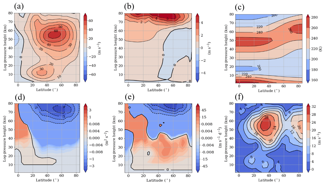
Figure 1Zonal-mean monthly mean (a) zonal wind (m s−1), (b) meridional wind (m s−1), (c) temperature (K), (d) zonal GW fluxes (m2 s−2), (e) GW zonal wind acceleration (m s−1 d−1) and (f) SPW 1 amplitude (m s−1) for the Northern Hemisphere. Results refer to January conditions, and to the reference simulation.
GWs are parameterized using an updated Lindzen-type linear scheme (Lindzen, 1981; Jakobs et al., 1986) with multiple breaking levels allowed (Fröhlich et al., 2003; Jacobi et al., 2006). The GWs are initialized at 10 km altitude, where at each grid point 48 waves are initiated, which propagate in eight different directions. In each direction, GWs have six different phase speeds ranging from 5 to 30 m s−1. The GW amplitudes are implemented as zonal means with a global average vertical velocity perturbation of 1 cm s−1. The amplitudes are weighted using a prescribed latitude distribution, which is based on GW potential energy observations derived from GPS radio occultation measurements (Šácha et al., 2015; Lilienthal et al., 2017). More details on the model and the standard analysis procedures are given in Samtleben et al. (2019). Like in Samtleben et al. (2019), we performed a reference simulation (Ref) for January conditions, using 2000–2010 mean ERA-Interim reanalysis data for specifying the lower atmosphere dynamics. The Ref simulation results are shown in Fig. 1. Here, the January zonal-mean latitude–height distributions of zonal (a) and meridional (b) winds, temperature (c), zonal GW flux (d), zonal wind acceleration due to breaking GWs (e), and the zonal wind SPW 1 amplitude (f) are presented. These results are the same as shown by Samtleben et al. (2019) and are repeated here for the sake of completeness and to facilitate the interpretation of the sensitivity study results below. As Samtleben et al. (2019) already mentioned, the model reproduces the background parameters (zonal and meridional wind and temperature) well in comparison to, for example, CIRA-86 (Fleming et al., 1988) and URAP (Swinbank and Ortland, 2003) climatologies. Also, the GW flux and the SPW amplitude (slightly overestimated) distributions are similar to observations (Ern et al., 2016; Xiao et al., 2009).
2.2 Experiment description
GW breaking hotspots in the stratosphere lead to an additional energy and momentum transfer, which is connected to an increased GW drag. In order to simulate the effect of a GW hotspot, the zonal (GWDu) and meridional (GWDv) GW drag as well as the GW heating (GWDT) have to be modified. We therefore enhanced the GW drag locally after the spin-up period of the model (after 270 d) and let the model run for another 120 d as in the Ref simulation. Because GW drag observations are strongly limited (for the meridional component even more than for the zonal component), we had to qualitatively estimate the forcing of the local breaking GW hotspots to be able to represent them in our model. To first estimate the direction of the GW drag, Šácha et al. (2015) analyzed the horizontal wind field in the region of the observed H3 GW hotspot. According to the wind field and the assumption that the GWs are orographically induced, the zonal and meridional GW drag were chosen to be negative. On the basis of a sensitivity study, in which Šácha et al. (2016) used different kind of negative GW drag values, they evaluated the intensity of the local GW forcings and their effects in the middle atmosphere. They found that (i) the strongest impact on the middle atmospheric circulation is caused by the zonal GW drag, while the meridional GW drag is more negligible and (ii) the combination of GWD m s−1 d−1, GWD m s−1 d−1 and GWDT=0.05 K d−1 is a quite moderate forcing, which does not lead to a total breakdown of the simulated polar vortex. Based on the preliminary work, we chose the moderate GW forcing (GWD m s−1 d−1, GWD m s−1 d−1, GWDT=0.05 K d−1) for our sensitivity study. Owing to the nonlinear interactions between the background circulation and the GWs, the artificial GW forcing leads to changes in the background circulation, which in turn influences the GW propagation and breaking conditions, and consequently modifies the GW drag and its regional distribution. This feedback mechanism was partly eliminated by turning off the GW parameterization in the further experiments and by using the GW drag output of the Ref simulation, which was modified in the GW hotspot region. As a starting point for our experiments as in Samtleben et al. (2019), we first focused on the observed Asian GW breaking hotspot, which was approximated by an enhanced GW drag between 37.5–62.5∘ N, 118.1–174.3∘ E and 18–30 km. This simulation is referred to as the H3 simulation. The GWDu distribution of the Ref (Fig. 2a) and the H3 (Fig. 2b) simulation is shown in Fig. 2 for about 27 km altitude, averaged for the last 30 d of analysis (day 390–420). In this respect, after the GW enhancement the circulation in the middle atmosphere stabilizes within 20 model days (Šácha et al., 2016), so that we can be sure that the atmospheric conditions are quite constant during the last 30 d of the simulations. Because we are mainly focusing on steady states, we concentrate on these last 30 model days during the analysis of the experiments and neglect short-term variabilities. In the Ref simulation, the GWDu varies between −0.02 and +0.02 m s−1 d−1 in the H3 GW hotspot region. With the implementation of the H3 GW hotspot (Fig. 2b), the GWDu has risen up to −10 m s−1 d−1; i.e., the additional GW forcing exceeds the maximum westward (negative) value of the Ref simulation by a factor of 500. The mean GWDu within the H3 hotspot area of the H3 simulation is −10 m s−1 d−1 and therefore 3300 larger than the mean GWDu of the Ref simulation, which is about 0.003 m s−1 d−1. With respect to GWDv and GWDT, both are maximum (mean) 5 (100) times stronger than those in the Ref simulation. Although these differences caused by the additional GW forcing seem to be quite large, the zonal GW forcing is still moderate compared to estimations from observations, which can exceed 40 m s−1 d−1, and from GW parameterizations in this region (Šácha et al., 2018).
Based on the approach of Samtleben et al. (2019), we now extend the sensitivity study by displacing the observed Asian GW hotspot (H3) longitudinally around one latitude circle. We therefore fixed the latitude (37.5–62.5∘ N) and altitude (18–30 km) range as well as the longitudinal extent of 56.25∘ but varied the position of the GW hotspot from 22.5–78.75∘ E (H1) to 22.5∘ W–33.75∘ E (H8) in steps of 45∘. The other artificial GW hotspots are labeled in between by H2 through H7. The position of the simulated GW hotspots can be seen in Fig. 2a. Compared to the first sensitivity study of Samtleben et al. (2019) the longitudinal displacement captures real GW hotspots more realistically, which may be orographically induced by the Rocky mountains (H5), the Himalayas (H2) or the European mountains (H8), or which may be generated by jet sources in the polar front region (H1–H8). Because of the displacement along a fixed latitude belt, the size of the artificial GW hotspots remains the same in contrast to the latitudinal displacement in Samtleben et al. (2019). Thus, the forcings of the individual GW hotspots are similar and the effect of the GW hotspot only depends on the position. Potentially, it may also depend on the resolution but experiments with refined resolution (not shown here) did not significantly change the results because (i) we introduced the same GW forcing (same ratio of grid points with changed and unchanged GW drag), (ii) the circulation does not change dramatically (only a small weakening of the polar vortex) and (iii) we only consider large-scale processes in our analysis, which are not strongly affected by the resolution of the model.
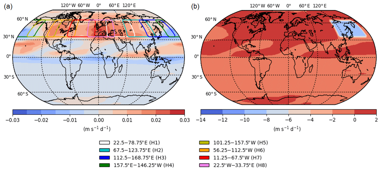
Figure 2Zonal GW drag (m s−1 d−1) at 26.9 km for the reference (a) and the H3 hotspot simulation (b). The last 30 model days are analyzed. Note the different scaling in panel (a).
3.1 GW hotspot effect on the background circulation
To analyze the GW hotspot effects on the middle atmosphere dynamics, the zonal-mean zonal wind and GW momentum flux differences between each GW hotspot H1–H8 (Fig. 3a–h) and the Ref simulation have been calculated. Both parameters, calculated by considering the last 30 model days, are shown in a latitude–height plot only for the Northern Hemisphere in Fig. 3. Most of the local GW hotspots cause a deceleration of the westerly wind northward of 40∘ N up to the lower mesosphere. The effect is strongest for the H6 hotspot, with 56.25–112.5∘ W longitudinal extent (Fig. 3f) with more than −20 m s−1. The weakest effect is seen for the H1 hotspot at 22.5–78.75∘ E, with only −4 m s−1 (Fig. 3a). However, the forcing is not strong enough to reverse the zonal-mean zonal wind and to produce a major SSW.
Owing to the weakening westerly wind, more eastward-directed GWs, traveling faster than the background wind, can partly propagate into the middle atmosphere and counteract the deceleration of the dominating westerly wind. This is underlined by the GW momentum flux, which is less negative, i.e., showing a positive difference, in the regions of negative zonal-mean zonal wind differences. The inversed effect is observed in regions of strengthening westerly wind (positive zonal wind differences) for nearly all of the experiments, and particularly expressed for the H1 (22.5–78.75∘ E) to H3 (118.1–174.3∘ E) hotspots, especially above 40 km altitude. This shows a decreased impact of eastward-directed GWs. Due to the increasing westerly wind in these regions, more eastward-directed GWs are filtered out (critical line) and the GW momentum flux becomes more negative. The negative (positive) zonal wind anomalies at higher (lower) latitudes mean that the polar vortex is strongly weakened and slightly shifted towards lower latitudes. The disturbance of the polar vortex can be also seen in the geopotential height and potential vorticity differences shown in polar plots in Fig. 4a–h. Both parameters have been averaged over the 20 to 30 km altitude range. The potential vorticity differences are given in color coding and the geopotential height differences are illustrated by the contour lines in intervals of 5 m with a highlighted zero line. Again, the dashed (solid) lines represent negative (positive) differences. The position of each GW hotspot is illustrated by a black box. The potential vorticity combines the conservation of vorticity and mass in the atmospheric system as well as the potential temperature for adiabatic processes. Because of the decreasing westerly wind and the destabilization of the polar vortex, the vorticity, which is normally increasing towards the polar region, is decreasing in each of the experiments. The decrease is strongest for the H3 (118.1–174.3∘ E) and H6 (56.25–112.5∘ W) GW hotspot in Fig. 4c and f and is mainly appearing at the northern flank of each GW hotspot. This is also the region of maximum geopotential height increase. Owing to the southward shift of the polar vortex, the potential vorticity is increasing in these regions. The increase is mostly occurring at the southern flank of the GW hotspot. The distribution of the potential vorticity anomalies can be explained by means of the quasi-geostrophic potential vorticity qg equation, considering that meridional GW drag is negligible compared to the zonal drag, and neglecting diabatic processes:
with Fx as the zonal GW drag. At the northern (southern) flank of the GW hotspot, is larger (smaller) than zero, so that is smaller (larger) than zero, which may explain the negative (positive) potential vorticity anomalies at the northern (southern) flank of the respective GW hotspots. The displacement of the polar vortex is connected with an increase in the geopotential height. However, in the region of the Aleutian high-pressure system, the geopotential height is decreasing. This effect can be observed for all GW hotspots and is most intense for the H3 (118.1–174.3∘ E) GW hotspot in Fig. 4c. As a result of the weakening of the Aleutian high, the polar vortex is less disturbed after the displacement towards lower latitudes. This corresponds to the strongest zonal-mean flow increase at lower latitudes up to 40 km in Fig. 3.
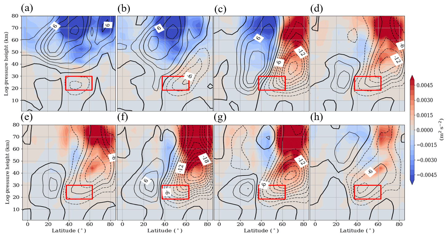
Figure 3Zonal-mean zonal wind (contour lines) and GW momentum flux (color coding) differences between the H1–H8 (a–h) and the Ref simulation. The last 30 model days are analyzed. Zonal wind differences are presented in intervals of 2 m s−1. The dashed (solid) lines represent negative (positive) differences. The zero line is highlighted. The position of the GW hotspots is shown by the red box.
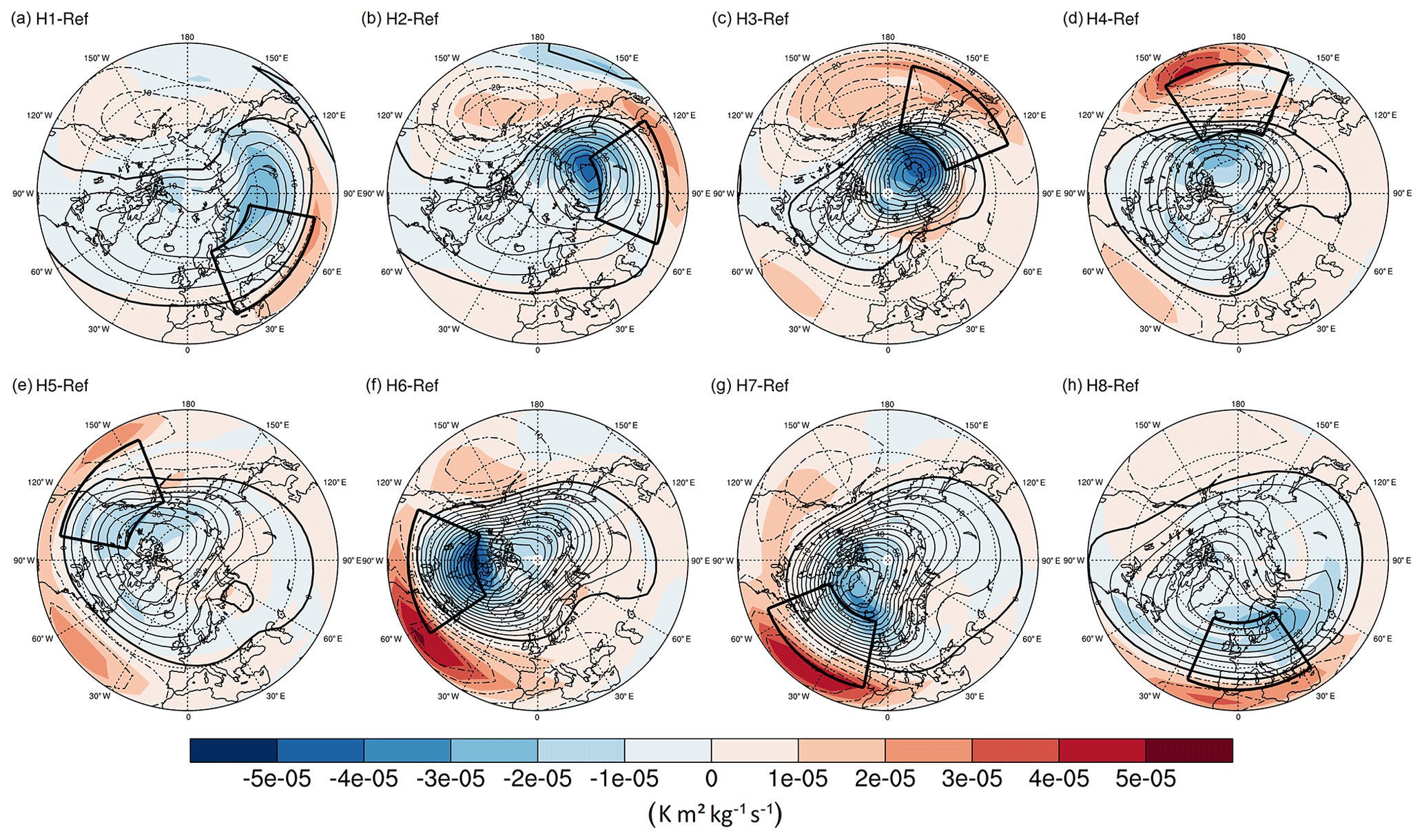
Figure 4Polar plots of the geopotential height (contour lines) and potential vorticity (color coding) differences between the H1–H8 (a–h) and the Ref simulation averaged between 20 and 30 km. Latitudes ranges from 30∘ N to the pole. Geopotential differences have a highlighted zero line and are presented in intervals of 5 m. The dashed (solid) line represents negative (positive) differences. The positions of the GW hotspots are illustrated by the black boxes.
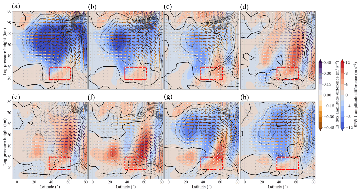
Figure 5Zonal-mean EP flux (arrows) and EP flux divergence (isolines, negative values are dashed) and zonal wind SPW 1 amplitude (color coding) differences between all H1–H8 (a–h) simulations and the reference simulation (H1–H8 – Ref). The positions of the GW hotspots are shown by red boxes.
3.2 Generation and propagation conditions of SPWs
The observed changes of the dynamics in the stratosphere and lower mesosphere and the related weakening of the polar vortex are mainly driven by the modulation of the SPWs. Figure 5 shows the zonal wind SPW 1 amplitude and the EP flux and divergence differences between each GW hotspot H1–H8 (panels a–h) and the Ref simulation results. The SPW 1 amplitude is strongly decreasing in the stratosphere and lower mesosphere for the H1 (22.5–78.75∘ E) to H3 (118.1–174.3∘ E) and the H7 (11.25–67.5∘ W) and H8 (22.5∘ W–33.75∘ E) GW hotspot; i.e., fewer SPWs 1 are propagating upward. This is in accordance with the decreasing EP flux and downward pointing arrows, underlining the fact that the SPWs 1 propagate less in the middle atmosphere. The effect is strongest for the H1 (22.5–78.75∘ E) GW hotspot with a SPW 1 amplitude decrease of more than −12 m s−1. These regions of decreased SPW 1 amplitude correspond to regions of strengthened zonal-mean westerly wind (Fig. 3). Due to the absent SPWs 1, fewer SPWs 1 are breaking, which leads to a reduced transfer of momentum and energy, and thus, to a less decelerated zonal wind. For this reason, we are observing a positive EP divergence difference showing that fewer SPWs are depositing their momentum. However, in comparison to the other GW hotspots, these GW hotspots (H1–H3, H7 and H8) generate new SPWs 1 in the lower mesosphere (positive EP flux divergence), which propagate further upward and also affect the mesosphere–lower thermosphere (MLT) region. The source of SPWs 1 can be seen in the positive EP divergence difference, the increased EP flux and the arrows pointing upward. In the H4–H6 GW hotspots the EP flux has increased in the high-latitude stratosphere–lower mesosphere. The arrows are directed upwards northward of 50∘ N up to about 70 km altitude, which means that more SPWs 1 are propagating into the middle atmosphere via the polar region. Some of these SPWs 1 are propagating into the middle atmosphere from the midlatitudes via the polar region, while some are directly generated in the polar region (positive EP divergence – source of SPWs 1). The increased SPWs 1 flux leads to increased SPW 1 amplitudes in the higher midlatitude stratosphere, which is strongest for the H6 (56.25–112.5∘ W) GW hotspot (Fig. 5f). Thus, more SPWs 1 are breaking, which amplifies the negative EP divergence and strongly decelerates the zonal-mean flow. This is consistent with the results in Fig. 3, which show a decreasing zonal-mean zonal wind at middle to high latitudes extending into the lower mesosphere. All simulations have in common that the SPW 1 amplitude is slightly decreasing at the southern as well as at the northern flank of each GW hotspot. This effect is more apparent by plotting the SPW 1 amplitude for a specific altitude of about 35 km in Fig. 6. To investigate to what extent the SPWs 2 and SPWs 3 are modified by the additional GW forcing, we also added their amplitudes in Fig. 6. As already shown in Fig. 5, the SPW 1 amplitude is strongest for the H6 (56.25–112.5∘ W, orange line) GW hotspot, with an increase of more than 12.5 m s−1. The H1 (22.5–78.75∘ E, black line) GW hotspot exhibits the strongest decrease in the SPW 1 amplitude of more than −14 m s−1. The SPW 1 anomalies owing to the GW hotspots can be separated into three groups: (I) H1 (22.5–78.75∘ E) and H2 (112.5–168.75∘ E), (II) H3 (118.1–174.3∘ E) and H8 (22.5∘ W–33.75∘ E), and (III) H4–H7. The SPW 1 amplitudes of the first group (I) mainly decrease in the whole winter hemisphere (WH) and only partly remain unchanged around 60∘ N. The minima of the SPW 1 differences are located between 40 and 50∘ N and in the polar region. The second group (II) shows increased SPW 1 amplitudes at 60∘ N (less than 4 m s−1) and decreased SPW 1 amplitudes (max. −7.5 m s−1) around 40 and 70∘ N. Although the SPW 1 anomalies of both hotspots are similar until 70∘ N, they diverge in the polar region, where the SPW 1 anomaly is positive for the H3 (118.1–174.3∘ E) and negative for the H8 (22.5∘ W–33.75∘ E) hotspot. Thus, the H8 (22.5∘ W–33.75∘ E) GW hotspot also exhibits features of the first group. The GW hotspots included in the third group (III) lead to increased SPW 1 amplitudes between 20 and 30∘ N, around 60∘ N and in the polar region. Compared to the second group, the increase in the SPW 1 amplitude is much stronger in the respective region. Around 40 and 70∘ N the SPW 1 amplitude decreases only slightly, except for the GW hotspot H7 (11.25–67.5∘ W), which shows a stronger decrease in the SPW 1 amplitude (comparable to the second group). However, nearly all of the SPW 1 differences show the same pattern with decreasing amplitudes around 40 and 70∘ N. From Samtleben et al. (2019) we already know that this pattern is not caused by the shape of the three-dimensional box with a sharp transition zone of changed and unchanged GW drag values. This pattern can be also partly observed in the SPW 2 amplitude anomalies. Compared to the SPW 1 amplitude anomalies, the SPW 2 anomalies are less variable and cannot really be separated into different groups. Thus, the SPW 2 is less affected by local GW hotspots. Only in case of the H7 (11.25–67.5∘ W, red line) and H8 (22.5∘ W–33.75∘ E) GW hotspots (violet line) has the SPW 2 amplitude slightly increased with more than 4 m s−1. Because the SPW 1 is highly dominating the middle atmosphere dynamics in the H6 (56.25–112.5∘ W) simulation, the SPW 2 amplitudes is strongly reduced by about −7.5 m s−1. For the H2–H5 GW hotspots, the SPW 2 anomalies show the same pattern as for the SPW 1 anomalies with decreasing amplitudes around 40 and 70∘ N (by less than −5 m s−1). With respect to the SPW 3 amplitude anomalies, it can be observed that the SPW 3 is not massively influenced by the different GW hotspots except for the lower latitudes, where the SPW 3 amplitude is partly decreasing by more than 5 m s−1 for the H3–H6 GW hotspots. To investigate whether the local GW forcings, which can be interpreted as an additional wave 1, are in or out of phase with those in the model, in Fig. 7 the zonal wind SPW 1 phase from the Ref simulation at an altitude of 27 km is shown as blue dots. Since the GW drag is negative (westward), we again define here the SPW 1 phase as the longitude of maximum westward wind. The colored boxes in Fig. 7 represent the longitudinal position of the local GW hotspots, here given in the range between 0 and 360∘ E. The superposition of two waves leads to a new wave with the same or larger (smaller) amplitude, if the phase difference of the two interfering waves ranges between 0 and ±120∘ (±120 and 180∘). For latitudes between 20 and 55∘ N, the phases of the SPW 1 (∼200∘) and the local GW forcing are similar (∼200∘ ± 120∘), if the local GW forcing is active between 80 and 320∘ (in longitudes 80–180∘ E and 40–180∘ W). This means in this latitude range, where the SPW 1 amplitude is usually largest (see Fig. 1f), the GW hotspots are in phase with the existing SPW 1, which might therefore be enhanced. This would correspond to the GW hotspots H3–H6, which are completely located in this range. Between 0 and 80∘ as well as between 320 and 360∘, the phase difference ranges between 120 and 240∘, which means that SPWs 1, which will be forced by the GW forcing in this region, interact destructively with the originally existing SPW 1. For this reason, GW hotspots such as the H1 (22.5–78.75∘ E) and H8 (22.5∘ W–33.75∘ E) ones do not influence the middle atmosphere dynamics that much by additional SPWs 1 as those of H3–H6. The H2 and H7 GW hotspots are partly in and out of phase with the SPWs 1 generated in the model. This corresponds to (i) the results of Fig. 4 showing that the polar vortex is more strongly disturbed by the H3–H6 GW hotspots (ii) as well as to the EP flux and SPW 1 amplitude differences, which are negative for the H1 (22.5–78.75∘ E) and H8 (22.5∘ W–33.75∘ E) GW hotspots and less negative or even positive for the H3–H6 GW hotspots.
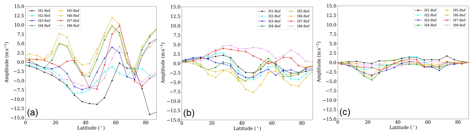
Figure 6Zonal-mean zonal wind SPW 1 (a), SPW 2 (b) and SPW 3 (c) amplitudes at 35 km altitude. Shown are differences between the H1–H8 and the Ref simulation.
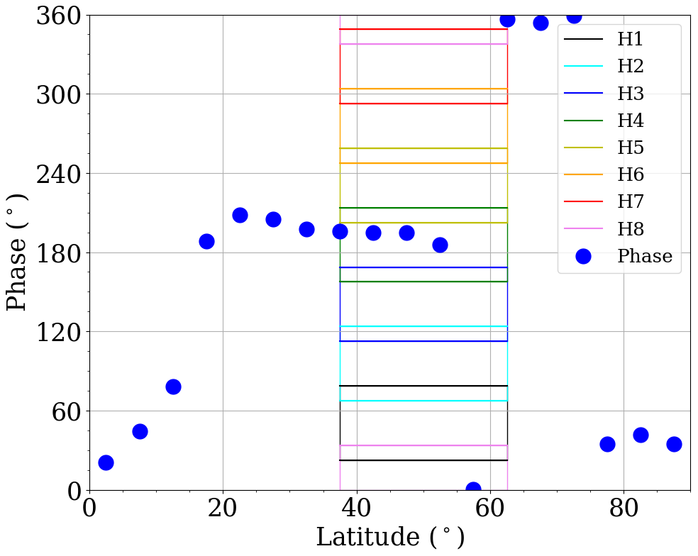
Figure 7Zonal wind SPW 1 phase of the Ref simulation (blue dots). The positions of the GW hotspots are illustrated by the colored boxes.
To investigate why SPWs 1 do not propagate into the middle atmosphere the refractive index n (Matsuno, 1971; Andrews et al., 1987) may be used. n strongly depends on the meridional potential vorticity gradient qy and on the zonal-mean zonal wind (Li et al., 2007). If n>0, wave propagation is possible. The larger n is, the higher the probability that waves are propagating into the upper atmosphere. SPWs are attracted by the regions of a large, positive n. For this reason SPWs mainly propagate upward and towards the Equator, where the zonal-mean flow is weak. For n<0 (easterly wind or strong westerly wind), the waves will break or will be reflected back to the troposphere and are not able to propagate (Matsuno, 1971). In Fig. 8 n was multiplied with the squared Earth radius. It shows the differences of n between the H2 (112.5–168.75∘ E, panel a) and H6 (56.25–112.5∘ W, panel b) simulations and the Ref simulations. The zero line as well as the negative n of the respective GW hotspot is indicated by the black line and the hatched area to show if negative differences refer to a negative or still positive n. In general, between 50 and 60∘ N, where the SPWs 1 usually propagate upwards, n is less positive or even negative (exceptions are H5 (101.25–157.5∘ W) and H8 (22.5∘ W–33.75∘ E)) in the region of the respective GW hotspot, as can be seen for the cases H2 (112.5–168.75∘ E) and H6 (56.25–112.5∘ W) in Fig. 8a and b. For this reason, fewer SPWs 1 propagate via the midlatitudes into the middle atmosphere, which corresponds to the decreasing EP flux in this region. In the polar region, where we observe increased SPW 1 amplitudes (H1–H8) and EP fluxes (H4–H6), n is increasing for all these simulations (not shown here). The effect is strongest for the H6 (56.25–112.5∘ W) simulation in Fig. 8b. Thus, the suppressed SPWs 1 from the midlatitudes are able to propagate into the polar region; i.e., the suppression is partly compensated. In most of the cases the SPWs 1 break there (negative EP divergence), because the propagation conditions are less suitable (H1–H3 and H7–H8). In turn, for the H4–H6 GW hotspots, the SPWs 1 are propagating from there further on into the middle atmosphere. While the SPWs of the H4 (157.5∘ E–146.25∘ W) and H5 (101.25–157.5∘ W) simulation propagate up to 70 km, those of the H6 (56.25–112.5∘ W) simulation are just going up to 50 km. In contrast to the H4 (157.5∘ E–146.25∘ W) and H5 (101.25–157.5∘ W) simulation, the H6 (56.25–112.5∘ W) simulation shows a strongly negative n anomaly (corresponding, in this case, to a negative n – hatched area) above the positive anomaly in the polar region (Fig. 8b), which means that the SPWs cannot travel further upward. Compared to the other simulations, the H1–H3 and the H7 GW hotspots generate SPWs 1 in the lower mesosphere propagating into the MLT region. Generally, n is negative in the upper mesosphere owing to the wind reversal (Samtleben et al., 2019). But due to the increasing westerly wind in this region, the propagation conditions change and n becomes positive, which can be seen around 80 km between 60 and 75∘ N in case of the H2 simulation (Fig. 8a). Local positive EP divergence anomalies connected with an increase in the SPW 1 amplitude and origin of the EP flux underline the generation of SPWs 1 in the polar region or lower mesosphere, for example. To see whether this might be an effect of local instabilities, we analyzed qy differences between the H2 (112.5–168.75∘ E, panel a) and H6 (56.25–112.5∘ W, panel b) simulations and the Ref simulations (Fig. 9b). The red boxes represent the latitude–height position of the GW hotspots. In accordance with the results of Samtleben et al. (2019), qy, which usually increases towards the polar region, reverses at the northern flank of each GW hotspot around 60∘ N due to the decreasing zonal-mean zonal wind and the connected weakening of the polar vortex. This negative qy anomaly (corresponding to a negative qy – hatched area) is strongest for the H6 (56.25–112.5∘ W) simulation in Fig. 9b, corresponding to the strongest zonal-mean zonal wind decrease. The local reversal of qy is an indicator for local instabilities (Charney and Stern, 1962) leading to the generation of nonstationary and stationary PWs. This may explain the locally enhanced SPW 1 amplitudes at the northern flank of each GW hotspot, which, however, are not able to propagate due to the unsuitable background conditions. While the negative qy as well as the anomaly of the H2 GW hotspot are locally limited around 60∘ N, that of the H6 simulation extends to the polar region. Thus, additional SPWs 1 are generated in the H6 simulation in the polar region (also enhanced positive EP divergence), where they are able to propagate further upwards and lead to the increased EP flux.
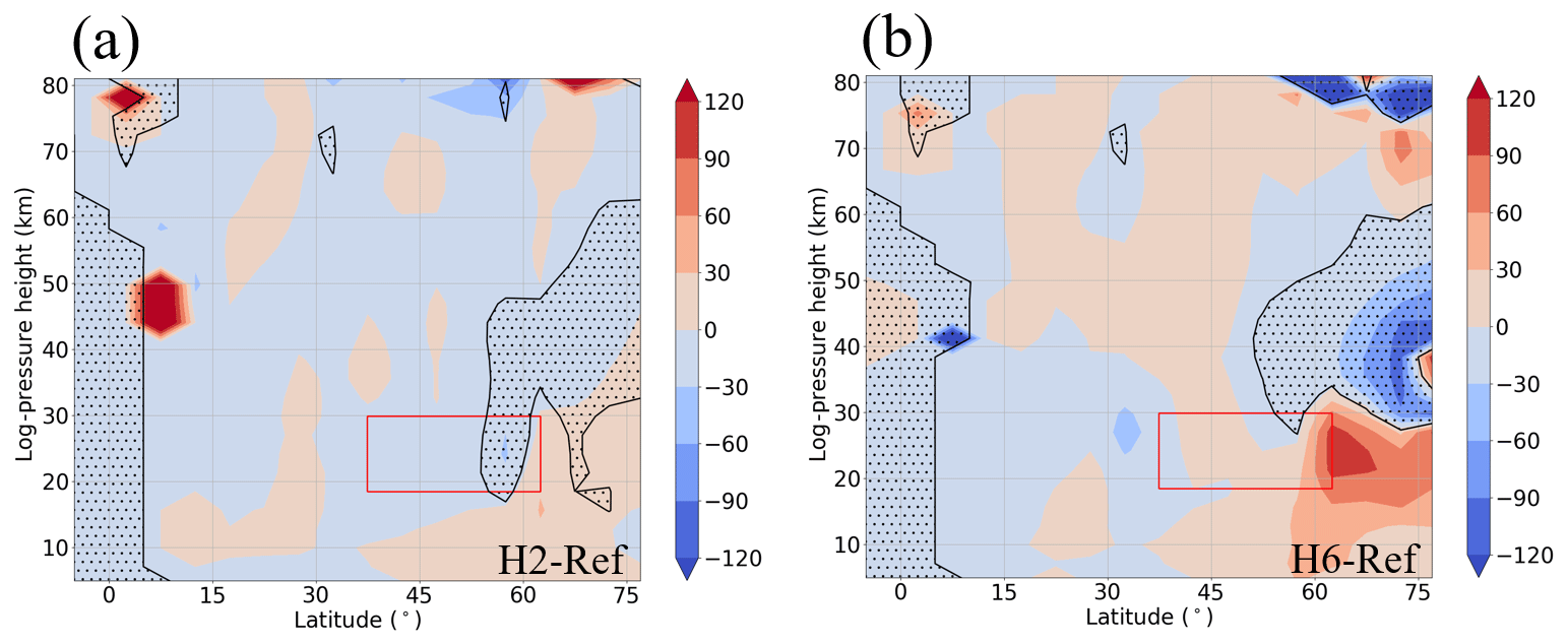
Figure 8Zonal-mean refractive index of SPW 1 differences between the H2 (a) and H6 (b) simulations and the Ref simulations. The hashed regions denote regions of negative refractive index of the H2 and H6 simulations. The positions of the GW hotspots are illustrated by the red boxes.
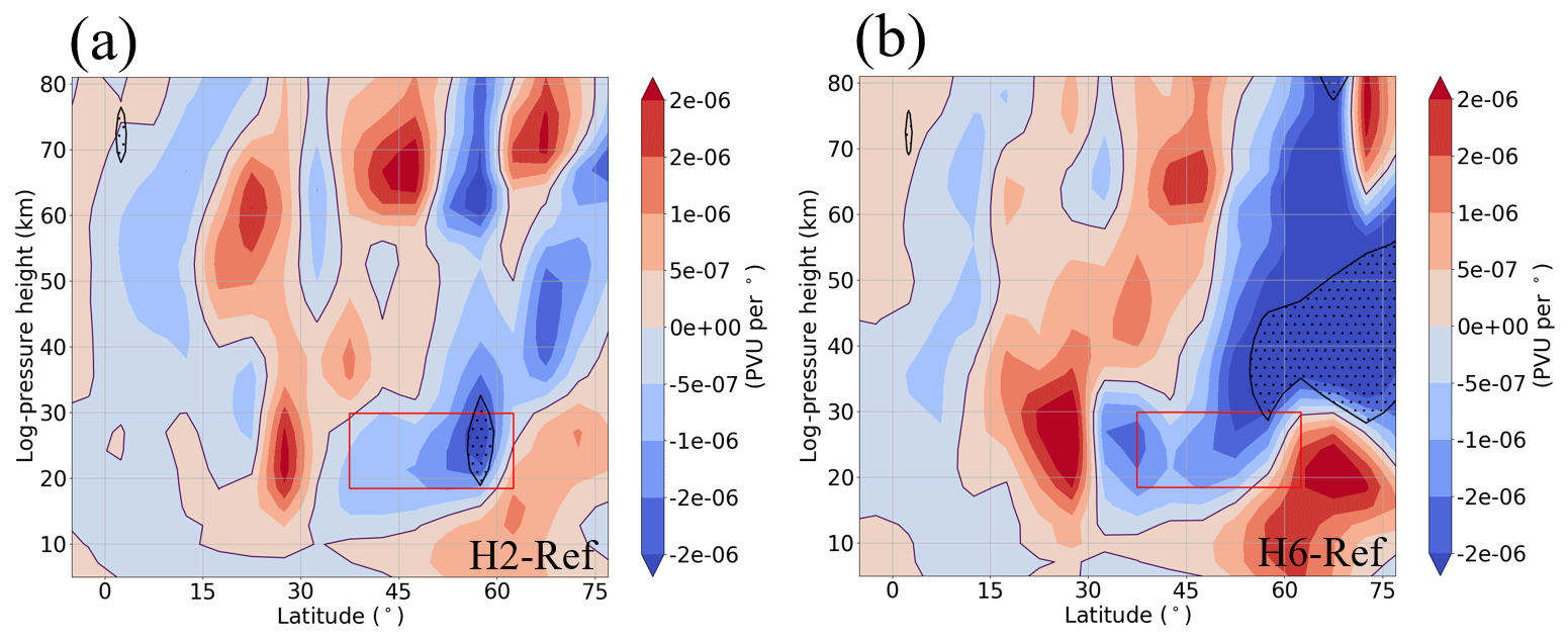
Figure 9Zonal-mean qy differences between the H2 (a) and H6 (b) simulations and the Ref simulations, given in potential vorticity units (PVU) per degree. The hashed regions denote regions of negative qy of the H2 and H6 simulations. The positions of the GW hotspots are shown by the red boxes.
As an extension of the results of Samtleben et al. (2019) we performed a continuing sensitivity study, which investigates the effect of breaking GW hotspots in the stratosphere and their impact on the middle atmosphere dynamics, which is mainly determined by the polar vortex. In contrast to Samtleben et al. (2019), we now focus on a fixed latitude range between 37.5 and 62.5∘ N and shift the artificial GW hotspot longitudinally in 45∘ steps, starting with the observed breaking GW hotspot located between 112.5 and 168.75∘ E. Strongly dependent on the position of the respective GW hotspot in relation to the phase of the SPW 1 generated in the model, the SPW 1 activity is either increasing or decreasing. Because the results are mostly determined by the phase of the SPW 1, we additionally compare the SPW 1 phase reproduced by the model (Fig. 10) to the SPW 1 phase extracted from SABER temperature measurements taken between 2002 and 2007 (Mukhtarov et al., 2010). To simplify the comparison, we choose the same latitude and altitude range as Mukhtarov et al. (2010) for the MUAM SPW 1 phase in Fig. 10. Since the measured 5-year mean SABER SPW 1 phase does not significantly change during the winter season, we are able to contrast the SABER SPW 1 phase from December (presented in Fig. 4 in Mukhtarov et al., 2010) with our modeled SPW 1 phase based on January conditions. The MUAM SPW 1 phase mostly corresponds to the SABER SPW 1 phase and is therefore quite realistic. We only find small differences, which may occur due to (i) the different time periods (2002–2007 for SABER and 2000–2010 for MUAM) or (ii) the different months (December for SABER and January for MUAM). Because the stability of the polar vortex is affected by the prevailing SPW activity, we observe scenarios in which the polar vortex is less or more weakened; i.e., the zonal-mean zonal wind is decreasing in connection with increased SPW 1 EP fluxes and negative divergences. In general, the local GW hotspots prevent the SPWs from propagating upwards at latitudes around 60∘ N, so that the SPWs propagate towards the polar region (positive n; Karami et al., 2016), where they are partly breaking and lead to the negative EP divergence decelerating the zonal-mean flow. In some cases, local instabilities indicated by the reversals in the qy also generate new SPWs 1 in the polar region (Charney and Stern, 1962; Garcia, 1991), which cause an additional transfer of momentum and energy. These local instabilities are also observed in the lower mesosphere, so that the SPWs 1 also have a lasting effect on the MLT region see (see Smith, 2003; Lieberman et al., 2013; Matthias and Ern, 2018). For those GW hotspots, which are in phase with the modeled SPW 1 and do not create a negative n in the upper polar region, the SPWs 1 propagate through the polar region further upward and influence the polar vortex up to an altitude of 70 km.
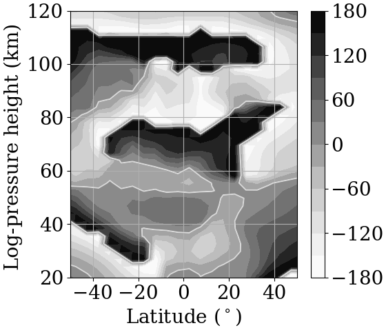
Figure 10Altitude–latitude cross section of the MUAM SPW 1 phase extracted from the temperature.
We briefly summarize the impact of each GW hotspot: the H1 (22.5–78.75∘ E) GW hotspot, which includes the Caucasus, the Ural mountains and the Anatolian plateau as possible orographic GW sources, produces an increase in zonal-mean flow above 40 km and only a slight decrease below. The increase in the zonal-mean flow is connected with a decrease in the SPW activity. This GW hotspot suppresses the SPW propagation at midlatitudes because it is out of phase with the SPW 1 originally generated in the model. It just slightly disturbs the polar vortex. The H2 (112.5–168.75∘ E) and H3 (118.1–174.3∘ E) GW hotspots, which include the Himalayas as possible orographic GW source (H2) and the Asian GW hotspot (H3), lead to decreasing (increasing) zonal-mean flow at middle to higher (low) latitudes, which is related to increasing (decreasing) SPW 1 amplitudes in the respective regions. Thus, the polar vortex is shifted southward. Both show a negative n at midlatitudes, preventing the SPWs from propagating upwards. The suppression of the SPWs is compensated for by additional wave propagation towards the polar region (increase in n), where they are breaking and maintain the deceleration of the polar vortex. Besides the destabilization, here the polar vortex displacement, the Aleutian high is also weakened (decrease in geopotential height). The effect of the H7 (11.25–67.5∘ W) and H8 (22.5∘ W–33.75∘ E) GW hotspots, which include the Alps and the Scandinavian Mountains, is similar. The H4-H6 GW hotspots, which include the Rocky Mountains, show a strong increase in the SPW 1 activity causing a strong deceleration of the zonal-mean flow at middle to higher latitudes. In contrast to the other simulations, the SPWs 1 can propagate into the middle atmosphere through the polar region, because they are in phase with the modeled SPW 1. The weakening of the Aleutian high pressure system is less intense for these three GW hotspots, so that the polar vortex is not only disturbed by the enhanced SPW activity but also by the Aleutian high pressure system. Besides the specified orographic sources, all H1–H8 GW hotspots may also include convective or jet sources.
In all of these experiments, we have observed changes in the geometry or even a strong preconditioning of the polar vortex, which make the polar vortex in reality more vulnerable for enhanced SPW activity and may lead to a SSW. Several studies based on satellite observations or reanalysis data (Albers and Birner, 2014; Ern et al., 2016) already reported increased GW activity in terms of an enhanced GW momentum flux and GW drag before SSW events, which would fit our basic idea for this sensitivity study. Because the effect strongly depends on the longitudinal position of the GW hotspot in relation to the phase of the modeled SPW 1, in future studies we will also focus on the influence of different atmospheric phenomena such as ENSO or NAO. The distribution of the SPW 1 phase may be strongly different for each phenomenon, so that some of the artificial GW hotspots can be in phase with the SPW 1 and would cause different effects than we have observed now. Additionally, instead of arbitrary positions of hotspots, their distribution should be more based on observations and known stable GW hotspots such as the Rocky Mountains or the Himalayas. Then, their analyzed impact and interaction will be more related to real atmospheric dynamical processes.
MUAM model code is available from the corresponding author upon request.
NS performed the model simulations and drafted the first version of the manuscript. PŠ provided the GW potential energy climatology. AK, PŠ, PP and CJ actively contributed to the discussions and the paper writing.
Christoph Jacobi is one of the Editors-in-Chief of Annales Geophysicae. The authors declare that they have no conflict of interest.
ERA-Interim reanalysis data have been provided by ECMWF through https://www.ecmwf.int/en/forecasts/datasets/browse-reanalysis-datasets (last access: 20 January 2020). We acknowledge support by Christoph Geißler, who performed MUAM simulations with a higher resolution to identify possible differences to our reference version.
This research has been supported by the Deutsche Forschungsgemeinschaft (DFG) (grant no. JA836/32-1) and the GA CR (grant nos. 16-01562J and 18-01625S).
This paper was edited by Gunter Stober and reviewed by two anonymous referees.
Albers, J. R. and Birner, T.: Vortex Preconditioning due to Planetary and Gravity Waves prior to Sudden Stratospheric Warmings, J. Atmos. Sci., 71, 4028–4054, https://doi.org/10.1175/JAS-D-14-0026.1, 2014. a, b
Andrews, D. G., Holton, J. R., and Leovy, C. B.: Middle Atmosphere Dynamics, ISBN 0-12-058576-6, Academic Press, San Diego, 1987. a, b
Beldon, C. L. and Mitchell, N. J.: Gravity wave-tidal interactions in the mesosphere and lower thermosphere over Rothera, Antarctica (68∘ S, 68∘ W), J. Geophys. Res.-Atmos., 115, D18101, https://doi.org/10.1029/2009JD013617, 2010. a
Charney, J. G. and Stern, M. E.: On the Stability of Internal Baroclinic Jets in a Rotating Atmosphere, J. Atmos. Sci., 19, 159–172, https://doi.org/10.1175/1520-0469(1962)019<0159:OTSOIB>2.0.CO;2, 1962. a, b
Costantino, L., Heinrich, P., Mzé, N., and Hauchecorne, A.: Convective gravity wave propagation and breaking in the stratosphere: comparison between WRF model simulations and lidar data, Ann. Geophys., 33, 1155–1171, https://doi.org/10.5194/angeo-33-1155-2015, 2015. a
Dee, D. P., Uppala, S. M., Simmons, A. J., Berrisford, P., Poli, P., Kobayashi, S., Andrae, U., Balmaseda, M. A., Balsamo, G., Bauer, P., Bechtold, P., Beljaars, A. C. M., van de Berg, L., Bidlot, J., Bormann, N., Delsol, C., Dragani, R., Fuentes, M., Geer, A. J., Haimberger, L., Healy, S. B., Hersbach, H., Hólm, E. V., Isaksen, L., Kallberg, P., Köhler, M., Matricardi, M., McNally, A. P., Monge-Sanz, B. M., Morcrette, J.-J., Park, B.-K., Peubey, C., de Rosnay, P., Tavolato, C., Thépaut, J.-N., and Vitart, F.: The ERA-Interim reanalysis: configuration and performance of the data assimilation system, Q. J. Roy. Meteor. Soc., 137, 553–597, https://doi.org/10.1002/qj.828, 2011. a
Douville, H.: Stratospheric polar vortex influence on Northern Hemisphere winter climate variability, Geophys. Res. Lett., 36, L18703, https://doi.org/10.1029/2009GL039334, 2009. a
Ern, M. and Preusse, P.: Gravity wave momentum flux spectra observed from satellite in the summertime subtropics: Implications for global modeling, Geophys. Res. Lett., 39, L15810, https://doi.org/10.1029/2012GL052659, 2012. a
Ern, M., Preusse, P., Alexander, M. J., and Warner, C. D.: Absolute values of gravity wave momentum flux derived from satellite data, J. Geophys. Res., 109, D20103, https://doi.org/10.1029/2004JD004752, 2004. a
Ern, M., Trinh, Q. T., Kaufmann, M., Krisch, I., Preusse, P., Ungermann, J., Zhu, Y., Gille, J. C., Mlynczak, M. G., Russell III, J. M., Schwartz, M. J., and Riese, M.: Satellite observations of middle atmosphere gravity wave absolute momentum flux and of its vertical gradient during recent stratospheric warmings, Atmos. Chem. Phys., 16, 9983–10019, https://doi.org/10.5194/acp-16-9983-2016, 2016. a, b, c
Fleming, E. L., Chandra, S., Barnett, J. J., and Corney, M.: Zonal mean temperature, pressure, zonal wind and geopotential height as functions of latitude, Adv. Space Res., 10, 11–59, https://doi.org/10.1016/0273-1177(90)90386-E, 1988. a
Fomichev, V. I. and Shved, G. M.: Parameterization of the radiative flux divergence in the 9.6 µm O3 band, J. Atmos. Terr. Phys., 47, 1037–1049, https://doi.org/10.1016/0021-9169(85)90021-2, 1985. a
Fomichev, V. I., Blanchet, J.-P., and Turner, D. S.: Matrix parameterization of the 15 mm CO2 band cooling in the middle and upper atmosphere for variable CO2 concentration, J. Geophys. Res., 103, 11505–11528, https://doi.org/10.1029/98JD00799, 1998. a
Fritts, D. C. and Alexander, M. J.: Gravity wave dynamics and effects in the middle atmosphere, Rev. Geophys., 41, 1003, https://doi.org/10.1029/2001RG000106, 2003. a, b
Fritts, D. C., Smith, R. B., Taylor, M. J., Doyle, J. D., Eckermann, S. D., Dörnbrack, A., Rapp, M., Williams, B. P., Pautet, P., Bossert, K., Criddle, N. R., Reynolds, C. A., Reinecke, P. A., Uddstrom, M., Revell, M. J., Turner, R., Kaifler, B., Wagner, J. S., Mixa, T., Kruse, C. G., Nugent, A. D., Watson, C. D., Gisinger, S., Smith, S. M., Lieberman, R. S., Laughman, B., Morre, J. J., Brown, W. O., Haggerty, J. A., Rockwell, A., Stossmeister, G. J., Williams, S. F., Hernandez, H., Murphy, D. J., Klekociuk, A. R., Reid, I. M., and Ma, J.: The deep propagation gravity wave experiment (DEEPWAVE): An airborne and ground-based exploration of gravity wave propagation and effects from their sources throughout the lower and middle atmosphere, B. Am. Meteorol. Soc., 97, 425–453, https://doi.org/10.1175/BAMS-D-14-00269.1, 2016. a, b
Fröhlich, K., Pogoreltsev, A., and Jacobi, C.: The 48-layer COMMA-LIM model, Rep. Inst. Meteorol. Univ. Leipzig, 30, 157–185, 2003. a
Fröhlich, K., Schmidt, T., Ern, M., Preusse, P., de la Torre, A., Wickert, J., and Jacobi, C.: The global distribution of gravity wave energy in the lower stratosphere derived from GPS data and gravity wave modelling: attempt and challenges, J. Atmos. Sol.-Terr. Phy., 69, 2238–2248, https://doi.org/10.1016/j.jastp.2007.07.005, 2007. a
Garcia, R. R.: Parameterization of planetary wave breaking in the middle atmosphere, J. Atmos. Sci., 48, 1405–1419, https://doi.org/10.1175/1520-0469(1991)048<1405:POPWBI>2.0.CO;2, 1991. a
Gisinger, S., Dörnbrack, A., Matthias, V., Doyle, J., Eckermann, S. D., Ehard, B., Hoffmann, L., Kaifler, B., Kruse, C. G., and Rapp, M.: Atmospheric conditions during the Deep Propagation Gravity Wave Experiment (DEEPWAVE), Mon. Weather Rev., 145, 4249–4275, https://doi.org/10.1175/MWR-D-16-0435.1, 2017. a
Hoffmann, L., Xue, X., and Alexander, M. J.: A global view of stratospheric gravity wave hotspots located with Atmospheric Infrared Sounder observations, J. Geophys. Res., 118, 416–434, https://doi.org/10.1029/2012JD018658, 2013. a, b, c
Hoffmann, P., Jacobi, C., and Borries, C.: Possible planetary wave coupling between the stratosphere and ionosphere by gravity wave modulation, J. Atmos. Sol.-Terr. Phys., 75–76, 71–80, https://doi.org/10.1016/j.jastp.2011.07.008, 2012. a
Jacobi, C., Fröhlich, K., and Pogoreltsev, A.: Quasi two-day-wave modulation of gravity wave flux and consequences for the planetary wave propagation in a simple circulation model, J. Atmos. Sol.-Terr. Phys., 68, 283–292, https://doi.org/10.1016/j.jastp.2005.01.017, 2006. a, b
Jakobs, H. J., Bischof, M., Ebel, A., and Speth, P.: Simulation of gravity wave effects under solstice conditions using a 3-D circulation model of the middle atmosphere, J. Atmos. Terr. Phys., 48, 1203–1223, https://doi.org/10.1016/0021-9169(86)90040-1, 1986. a
Karami, K., Braesicke, P., Sinnhuber, M., and Versick, S.: On the climatological probability of the vertical propagation of stationary planetary waves, Atmos. Chem. Phys., 16, 8447–8460, https://doi.org/10.5194/acp-16-8447-2016, 2016. a
Li, Q., Graf, H.-F., and Giorgetta, M. A.: Stationary planetary wave propagation in Northern Hemisphere winter – climatological analysis of the refractive index, Atmos. Chem. Phys., 7, 183–200, https://doi.org/10.5194/acp-7-183-2007, 2007. a
Lieberman, R. S., Riggin, D. M., and Siskind, D. E.: Stationary waves in the wintertime mesosphere: Evidence for gravity wave filtering by stratospheric planetary waves, J. Geophys. Res., 118, 3139–3149, https://doi.org/10.1002/jgrd.50319, 2013. a
Lilienthal, F., Jacobi, C., Schmidt, T., de la Torre, A., and Alexander, P.: On the influence of zonal gravity wave distributions on the Southern Hemisphere winter circulation, Ann. Geophys., 35, 785–798, https://doi.org/10.5194/angeo-35-785-2017, 2017. a, b
Lilienthal, F., Jacobi, C., and Geißler, C.: Forcing mechanisms of the terdiurnal tide, Atmos. Chem. Phys., 18, 15725–15742, https://doi.org/10.5194/acp-18-15725-2018, 2018. a
Lindzen, R. S.: Turbulence and stress owing to gravity wave and tidal breakdown, J. Geophys. Res., 86, 9707–9714, https://doi.org/10.1029/JC086iC10p09707, 1981. a
Manson, A., Meek, C., Luo, Y., Hocking, W., MacDougall, J., Riggin, D., Fritts, D., and Vincent, R.: Modulation of gravity waves by planetary waves (2 and 16 d): observations with the North American-Pacific MLT-MFR radar network, J. Atmos. Sol.-Terr. Phy., 65, 85–104, https://doi.org/10.1016/S1364-6826(02)00282-1, 2003. a
Matsuno, T.: A dynamical model of the stratospheric sudden warming, J. Atmos. Sci., 28, 1479–1494, https://doi.org/10.1175/1520-0469(1971)028<1479:ADMOTS>2.0.CO;2, 1971. a, b
Matthias, V. and Ern, M.: On the origin of the mesospheric quasi-stationary planetary waves in the unusual Arctic winter 2015/2016, Atmos. Chem. Phys., 18, 4803–4815, https://doi.org/10.5194/acp-18-4803-2018, 2018. a
Miyahara, S. and Forbes, J. M.: Interactions between gravity waves and the diurnal tide in the mesosphere and lower thermosphere, J. Meteorol. Soc. Jpn. Ser. II, 69, 523–531, https://doi.org/10.2151/jmsj1965.69.5_523, 1991. a
Mukhtarov, P., Pancheva, D., and Andonov, B.: Climatology of the stationary planetary waves seen in the SABER/TIMED temperatures (2002–2007), J. Geophs. Res., 115, A06315, https://doi.org/10.1029/2009JA015156, 2010. a, b, c
Nastrom, G. D. and Fritts, D. C.: Sources of mesoscale variability of gravity waves. Part I: Topographic Excitation, J. Atmos. Sci., 49, 101–110, https://doi.org/10.1175/1520-0469(1992)049<0101:SOMVOG>2.0.CO;2, 1992. a
Plougonven, R. and Zhang, F.: Internal gravity waves from atmospheric jets and fronts, Reviews of Geophysics, American Geophysical Union, 52, 33–76, https://doi.org/10.1002/2012RG000419, 2014. a, b
Plougonven, R., Hertzog, A., and Teitelbaum, H.: Observations and simulations of a large-amplitude mountain wave breaking over the Antarctic Peninsula, J. Geophys. Res., 113, D16113, https://doi.org/10.1029/2007JD009739, 2008. a
Pogoreltsev, A. I., Vlasov, A. A., Fröhlich, K., and Jacobi, C.: Planetary waves in coupling the lower and upper atmosphere, J. Atmos. Sol.-Terr. Phy., 69, 2083–2101, https://doi.org/10.1016/j.jastp.2007.05.014, 2007. a
Preusse, P., Eckermann, S., Oberheide, J., Hagan, M., and Offermann, D.: Modulation of gravity waves by tides as seen in CRISTA temperatures, Adv. Space Res., 27, 1773–1778, https://doi.org/10.1016/S0273-1177(01)00336-2, 2001. a
Šácha, P., Kuchař, A., Jacobi, C., and Pišoft, P.: Enhanced internal gravity wave activity and breaking over the northeastern Pacific–eastern Asian region, Atmos. Chem. Phys., 15, 13097–13112, https://doi.org/10.5194/acp-15-13097-2015, 2015. a, b, c, d
Šácha, P., Lilienthal, F., Jacobi, C., and Pišoft, P.: Influence of the spatial distribution of gravity wave activity on the middle atmospheric dynamics, Atmos. Chem. Phys., 16, 15755–15775, https://doi.org/10.5194/acp-16-15755-2016, 2016. a, b, c, d
Šácha, P., Miksovsky, J., and Pisoft, P.: Interannual variability in the gravity wave drag – vertical coupling and possible climate links, Earth Syst. Dynam., 9, 647–661, https://doi.org/10.5194/esd-9-647-2018, 2018. a
Samtleben, N., Jacobi, C., Pišoft, P., Šácha, P., and Kuchař, A.: Effect of latitudinally displaced gravity wave forcing in the lower stratosphere on the polar vortex stability, Ann. Geophys., 37, 507–523, https://doi.org/10.5194/angeo-37-507-2019, 2019. a, b, c, d, e, f, g, h, i, j, k, l, m, n, o, p, q, r, s
Scheffler, G., Pulido, M., and Rodas, C.: The role of gravity wave drag optimization in the splitting of the Antarctic vortex in the 2002 sudden stratospheric warming, Geophys. Res. Lett., 45, 6719–6725, https://doi.org/10.1029/2018GL077993, 2018. a, b
Schmidt, T., Alexander, P., and de la Torre, A.: Stratospheric gravity wave momentum flux from radio occultations, J. Geophys. Res., 121, 4443–4467, https://doi.org/10.1002/2015JD024135, 2016. a
Senf, F. and Achatz, U.: On the impact of middle-atmosphere thermal tides on the propagation and dissipation of gravity waves, J. Geophys. Res.-Atmos., 116, D24110, https://doi.org/10.1029/2011JD015794, 2011. a
Smith, A. K.: The origin of stationary planetary waves in the upper mesosphere, J. Atmos. Sci., 60, 3033–3041, https://doi.org/10.1175/1520-0469(2003)060<3033:TOOSPW>2.0.CO;2, 2003. a
Smith, R. B.: On severe downslope winds, J. Atmos. Sci., 42, 2597–2603, https://doi.org/10.1175/1520-0469(1985)042<2597:OSDW>2.0.CO;2, 1985. a
Strobel, D. F.: Parameterization of the atmospheric heating rate from 15 to 120 km due to O2 and O3 Absorption of solar radiation, J. Geophys. Res., 83, 6225–6230, https://doi.org/10.1029/JC083iC12p06225, 1986. a
Swinbank, R. and Ortland, D. A.: Compilation of wind data for the Upper Atmosphere Research Satellite (UARS) Reference Atmosphere Project, J. Geophys. Res., 108, 4615, https://doi.org/10.1029/2002JD003135, 2003. a
Tsuda, T., Muayama, Y., Wiryosumarto, H., Harijono, S. W. B., and Kato, S.: Radiosonde observations of equatorial atmosphere dynamics over Indonesia. II: characteristics of gravity waves, J. Geophys. Res., 99, 10507–10516, https://doi.org/10.1029/94JD00354, 1994. a
Xiao, C., Hu, X., and Tian, J.: Global temperature stationary planetary waves extending from 20 to 120 km observed by TIMED/SABER, J. Geophys. Res., 114, D17101, https://doi.org/10.1029/2008JD011349, 2009. a