the Creative Commons Attribution 4.0 License.
the Creative Commons Attribution 4.0 License.
 | 17 Jan 2020
Evidence of vertical coupling: meteorological storm Fabienne on 23 September 2018 and its related effects observed up to the ionosphere
Petra Koucká Knížová
Kateřina Podolská
Kateřina Potužníková
Daniel Kouba
Zbyšek Mošna
Josef Boška
Michal Kozubek
A severe meteorological storm system on the frontal border of cyclone Fabienne passing above central Europe was observed on 23–24 September 2018. Large meteorological systems are considered to be important sources of the wave-like variability visible/detectable through the atmosphere and even up to ionospheric heights. Significant departures from regular courses of atmospheric and ionospheric parameters were detected in all analyzed datasets through atmospheric heights. Above Europe, stratospheric temperature and wind significantly changed in coincidence with fast frontal transition (100–110 km h−1). Zonal wind at 1 and 0.1 hPa changes from the usual westward before the storm to eastward after the storm. With this change are connected changes in temperature where at 1 hPa the analyzed area is colder and at 0.1 hPa warmer. Within ionospheric parameters, we have detected significant wave-like activity occurring shortly after the cold front crossed the observational point. During the storm event, both by Digisonde DPS-4D and continuous Doppler sounding equipment, we have observed strong horizontal plasma flow shears and time-limited increase plasma flow in both the northern and western components of ionospheric drift. The vertical component of plasma flow during the storm event is smaller with respect to the corresponding values on preceding days.
The analyzed event of an exceptionally fast cold front of cyclone Fabienne fell into the recovery phase of a minor–moderate geomagnetic storm observed as a negative ionospheric storm at European mid-latitudes. Hence, ionospheric observations consist both of disturbances induced by moderate geomagnetic storms and effects originating in convective activity in the troposphere. Nevertheless, taking into account a significant change in the global circulation pattern in the stratosphere, we conclude that most of the observed wave-like oscillations in the ionosphere during the night of 23–24 September can be directly attributed to the propagation of atmospheric waves launched on the frontal border (cold front) of cyclone Fabienne. The frontal system acted as an effective source of atmospheric waves propagating upward up to the ionosphere.


The ionosphere is a highly variable system that is influenced by solar and geomagnetic activity from above and lower-laying atmospheric phenomena from below. Ionospheric variability is observed on a wide-scale range from minutes, or even shorter, up to scales of the solar cycle and secular variations of solar energy input. Without doubt, the most dominant driver of ionospheric variability is solar activity. The whole atmosphere and ionosphere react according to the level of solar energy input. The episodes of limited strongly enhanced dissipation of solar energy (solar flares, coronal mass ejections, etc.) can affect only regions localized at high latitudes or can cover all of the geosphere. During such an event, the magnetosphere is affected first (see for instance Hargreaves, 1992). A large portion of solar energy is dissipated in the upper atmosphere and then in the ionosphere and thermosphere (Davies, 1990; Solomon and Qian, 2005). The perturbations can be detected at the ground level, for instance by magnetometers. Disturbances associated with such enhanced solar energy inputs are in general called geomagnetic storms (Gonzales et al., 1994; Buonsanto, 1999) or geospheric storms (Prölss, 2004). Different types of solar agents that are mainly responsible for geomagnetic disturbances have been analyzed with respect to their geoeffectiveness by Kakad et al. (2019), Georgieva et al. (2006), Fenrich and Luhmann (1998), Leamon et al. (2002), Prölss (2004) and many others.
Besides the solar and geomagnetic forcing, the energy inputs from lower-laying atmospheric heights must be taken into account in the energy budget of the ionosphere. The lower-laying atmosphere and its impact on the ionosphere have largely been studied during the last exceptionally low solar cycle by means of a growing number of satellite measurements. A paper by Anthes (2011) and a more recent paper by Liu at al. (2017) demonstrated the effectivity of radio occultation (RO) sounding methods onboard satellites for systematic sounding of the atmosphere with respect to weather, climate and space weather.
The ionosphere is weakly ionized plasma where both neutrals and ions play an important role. Ionization degree around the maximum of electron concentration is less than 10−2 and significantly smaller below the maximum in the F layer, except for limited events of sporadic E-layer occurrence (Whitehead, 1961, 1990; Mathews, 1998; Haldoupis, 2012). The impact of the collision processes on the ionospheric dynamics cannot be neglected, especially in the lower ionosphere. During day time, due to incoming solar radiation, the ionosphere is formed at the height of the mesosphere and thermosphere. The ionosphere is typically stratified into D, E and F layers, where the maximum electron concentration is usually located. The F layer is usually a region with maximum electron concentration. It can be split into two sublayers denoted the F1 and F2 layers. In the case of splitting into F1 and F2 layers, the maximum of the electron concentration is located in the F2 layer. During night time electron concentration decreases at all heights due to recombination processes and a lack of ionizing radiation. It leads to practical disappearance of all ion pairs below the F layer that remains present due to slow recombination processes at its height (Davies, 1990; Rishbeth, 1998; Prölss, 2004, among many others). As a measure of the ability of the Earth's atmosphere to absorb incoming solar radiation, we can consider the maximum electron concentration NmF2 in the highest ionospheric level F or F2 if present. During the solar cycle, we can observe a clear link between incoming solar radiation and ionospheric ionization. With the increasing solar activity we observe higher ionization. However, the relationship is not linear and is the subject of a large investigation. The link between ionospheric variability and both solar and geomagnetic indices was analyzed for instance by Clilverd et al. (2003), Cnossen et al. (2014), Forbes et al. (2000), Roux et al. (2012), Koucká Knížová et al. (2018), and Perrone et al. (2017). Understanding of the relation between solar activity and the corresponding ionospheric and/or atmospheric behavior is crucial for instance in the estimation of the trends and potential human impact on the atmosphere and ionosphere (Roininen et al., 2015; Laštovička et al., 2012; Laštovička, 2012; Georgieva et al., 2012).
The ionosphere clearly reflects solar activity on all studied timescales. Diurnal courses of the maximum concentration in the ionosphere clearly show the dominant solar influence, increase/decrease in the electron concentration with respect to the solar zenith angle. During stable solar and geomagnetic situations, however, a significant difference in the courses of ionospheric parameters is well seen on consequent days. Vertically propagating gravity waves have been the subject of great scientific interest since the 1960s. A fundamental interpretation of atmospheric variability in terms of atmospheric gravity waves was provided by Hines (1960) and later by Hines (1963, 1965, and 1968). The effects of gravity waves on the ionosphere up to the F2 region through photochemical and dynamical processes were discussed by Hooke (1970b). Garcia and Solomon (1985) reported gravity wave importance for the chemical composition of the middle atmosphere. There, it was already shown that the resulting effects of gravity waves depend not only on the wave properties, but also on the actual ionospheric situation and/or the direction of propagation with respect to incoming solar radiation (Hooke, 1970a, 1971). It has been pointed out by Holton (1983) that gravity-wave drag and diffusion are fundamental for the wind and temperature balance in the middle atmosphere. Fritts and Nastrom (1992) suggested that convective activity in the troposphere is as important a source of gravity waves as topographic forcing. Model study of gravity-wave generation and its observable signatures above deep convection is provided by Alexander et al. (1994). Tropospheric convective systems are often connected with strong lightning. The possibility of thunderstorm influence on the ionosphere has already been suggested by Bhar and Syam (1937). In general, two principal mechanisms are proposed. The first mechanism presumes gravity waves generated by thunderstorms to propagate up to ionospheric heights. The second mechanism involves generation of electrical discharges in the E region above the storm. Applying superposed epoch analyses, Davis and Johnson (2005) reported statistically significant intensification and descent in altitude of the mid-latitude sporadic E layer directly above the thunderstorm. Different observational results showing a decrease in the critical frequency of sporadic E have been reported by Barta et al. (2017). The mechanism involved in the coupling between thunderstorm lightning and ionosphere is very complicated and not well understood yet. The limitations of generally accepted mechanisms are discussed in detail in the paper by Haldoupis (2018).
Later detailed model studies of gravity-wave propagation through the Earth's atmosphere simulations provided by Vadas and Fritts (2005), Vadas (2007), and Vadas and Nicolls (2012) proved that gravity waves originating in the tropospheric convection can reach thermospheric heights and significantly affect wind and temperature profiles. Atmospheric waves propagate from the lower-laying atmosphere up to the thermosphere as primary waves or dissipate. The deposited momentum excites secondary waves (see for instance Vadas and Liu, 2009, or Vadas et al., 2018).
Except for model studies there are observational evidences of consequent ionospheric disturbances attributed to dynamical processes in the lower atmosphere. Chernigovskaya et al. (2018) provide evidence of an F2-layer ionospheric response to dynamic processes during the winter circumpolar vortex evolution in the strato-mesosphere. McDonald et al. (2018) reported an enhancement in total electron content in the ionosphere, which coincides with the commencement of a stratospheric warming event. Goncharenko et al. (2010) observed persistent variations in the low-latitude ionosphere that occur several days after a sudden warming event in the high-latitude winter stratosphere. Enhancements of wave-like activity within the ionospheric F layer with relation to meteorological events were reported by Chernigovskaya et al. (2015). Propagation of concentric gravity waves from the source region in the troposphere related to tropospheric convective storms up to the ionosphere was reported by Azeem et al. (2015). This paper presents almost simultaneous observations of a gravity-wave event in the stratosphere, mesosphere, and ionosphere. Suddenly increasing wave-like oscillations within ionospheric parameters after passing a tropospheric cold front across an observational point were reported by Boška and Šauli (2001) and Šauli and Boška (2001). On the longer-term scale, the extremely high correlation between ionospheric measurements up to the “break point” at 10 degrees in longitude and/or Earth's distance of 1000 km is attributed to the mesoscale systems as proposed by Koucká Knížová et al. (2015). Infrasound waves excited by severe tropospheric storms (e.g., typhoons and strong storms) are discussed and analyzed. Chum et al. (2018) detected infrasound in the ionosphere from earthquakes and typhoons by means of multi-point continuous Doppler sounding equipment. The authors give examples of observation by an international network of continuous Doppler sounders. The waves were observed at the height range from about 200 to 300 km by a continuous Doppler sounder located in Taiwan (Chum et al., 2018). The infrasound was observed during several hours for strong storm events.
GPS satellite measurements are promising tools for monitoring ionospheric changes connected with severe weather systems. Recently the analyses of the scintillation S4 index in relation to four tropical cyclones (Yasi in 2011, Marcia in 2015, Debbie in 2017 and Marcus in 2018) were presented by Ke et al. (2019). They found intensification of scintillation effects mostly above the tropical cyclone path and attributed them to the electric field perturbation and consequent plasma bubble generation. Within COSMIC GPS data, Yang and Liu (2016) found a significant peak in radio occultation scintillation events during the passage of tropical cyclone Tembin in 2012 during quiet geomagnetic or solar activity and attributed the observed effect to the gravity waves generated in the lower atmosphere by the cyclone. Afraimovich et al. (2013) published a large review of GPS/GLONASS studies of the ionospheric response to natural and anthropogenic processes and phenomena. This paper focuses on a wide range of ionospheric forcing and corresponding ionospheric variability detected in principle within total electron content (TEC) and F2-layer critical frequency foF2. In relation to tropical cyclones (Katrina, Rita and Wilma) occurring in 2005, they reported an increase in wave-like activity in the gravity-wave period range mainly in the range 20 to 60 min and intensification of TEC variations along the satellite path close to the cyclone. The zones of disturbances were found to form during the hurricane stage of the cyclone (Afraimovich et al., 2013).
Review of lower atmosphere forcing was provided by Lastovička (2006). Review of coupling processes in the atmosphere with respect to atmospheric waves and sudden stratospheric warmings can be found in Yigit et al. (2016). The importance of involvement of the lower atmosphere in ionospheric variability studies in order to accurately capture smaller-scale features of the upper atmosphere response even to the geomagnetic storms is demonstrated by Pedatella and Liu (2018). The evidence of lower atmosphere forcing is clearly demonstrated in the day-to-day ionospheric variability (known as an ionospheric anomaly) during low and stable solar and geomagnetic activity during subsequent days. Ionospheric parameters (e.g., electron concentration or height of ionospheric layers) on such scales are influenced by a combination of meteorologic activity and solar/geomagnetic forcing. During geomagnetically quiet days the tropospheric forcing is more emphasized and relatively more important and rules the ionospheric dynamics, far more than the solar and geomagnetic energy inputs.
The model study (Pedatella and Liu, 2018) demonstrated variability of the response of the atmosphere and ionosphere system to one particular storm when the internal variability characterized by the ensemble standard deviation is introduced. The study shows that implementation of arbitrary internal atmospheric variability leads to the geomagnetic storm occurring under a different, though climatically similar, atmospheric state for each ensemble member. The study has found that variability leads to an uncertainty of typically 20 %–40 %, with localized regions exceeding 100 %. It clearly shows that large-scale features of the storm are reproduced well and that small-scale characteristics of the response are dependent on lower atmosphere variability. Hence neglecting the lower atmosphere may lead to significant complication in the geomagnetic storm interpretation.
For the description of cyclone Fabienne in the troposphere we use meteorological ground-based data (https://www.ventusky.com/, last access: 3 October 2018, https://www.wetterkontor.de, last access: 3 October 2018, http://wetter3.de, last access: 3 October 2018, http://www.ufa.cas.cz/institute-structure/department-of-meteorology/present-weather-sporilov.html, last access: 3 October 2018) and Aeolus satellite measurements described in the following Sect. 2.1. Behavior of the stratosphere is interpreted using stratospheric wind and temperature reanalysis MERRA-2 datasets (https://disc.gsfc.nasa.gov/daac-bin/FTPSubset2.pl, last access: 15 November 2018) described in Sect. 2.2. The ionosphere observation (details are provided in Sect. 2.3) comes from two ground-based vertical ionospheric soundings using the Digisonde DPS-4D (http://giro.uml.edu/, last access: 26 November 2018 and http://digisonda.ufa.cas.cz/, last access: 26 November 2018) and oblique reflection using the multi-point continuous Doppler sounding (CDS) http://www.ufa.cas.cz/files/OHA/M_Doppler_system.pdf, last access: 22 October 2018. Besides that we use satellite TEC measurement (http://gnss.be/Atmospheric_Maps/ionospheric_maps.php, last access: 10 October 2018) for station Pruhonice. For geomagnetic situation description we use geomagnetic indices from Potsdam Data Center (https://www.gfz-potsdam.de/en/kp-index/, last access: 21 November 2018). The data used for interpretation of the Fabienne event and related disturbances in stratospheric and ionospheric heights cover the time interval 20–27 September 2018.
2.1 Meteorological data
In order to describe severe storm Fabienne, we use ground-based meteorological monitoring combined with satellite observation. For determination of the synoptic condition in the troposphere, surface and upper synoptic maps were used (available at https://www.wetterkontor.de/, last access: 3 October 2018 and http://wetter3.de, last access: 3 October 2018). We also used meteorological ground-based radar observations taken from https://www.ventusky.com/ (last access: 3 October 2018). In addition, hourly averaged meteorological data performed by the automatic weather station located at the Institute of Atmospheric Physics, IAP (50.04∘ N, 14.48∘ E), were used to determine the time of the frontal passage (http://www.ufa.cas.cz/institute-structure/department-of-meteorology/present-weather-sporilov.html, last access: 3 October 2018). Data are available for last 30 d and then they are stored in the institute's archive.
The Aeolus Earth Explorer Atmospheric Dynamics Mission yields data from global observations of wind profiles from space using the active Doppler wind lidar (DWL) method (Gompf, 2000). The DWL measurement is a unique method that has the potential to provide the required data on a global scale from direct observation of wind. The DWL measures 100 wind profiles per hour using both the Rayleigh and Mie scattering methods (Durand et al., 2004). The global wind profiles (along a single line-of-sight) are measured up to an altitude of 30 km to an accuracy of 1 m s−1 in the planetary boundary layer (up to an altitude of 2 km). The Aeolus mission was launched on 22 August 2018 and scientific measurement started on 12 September 2018.
2.2 Stratospheric data
The MERRA-2 (Modern-Era Retrospective analysis for Research and Applications, version 2 from https://disc.gsfc.nasa.gov/daac-bin/FTPSubset2.pl, last access: 15 November 2018) with resolution 0.5∘ in latitude and 2∕3∘ in longitude was used. The MERRA-2 is a global atmospheric reanalysis produced by the NASA Global Modelling and Assimilation Office (GMAO); details can be found in Gelaro et al. (2017). The MERRA-2 is available up to 0.1 hPa from 1980 till the present, but we show only 1 and 0.1 hPa for the period from 20 to 27 September 2018, which is relevant for our studies. This reanalysis provides reliable time series in a regular grid network. Temperature and zonal wind 6-hourly data (00:00, 06:00, 12:00 and 18:00 UT) in the stratosphere and lower mesosphere (from 30–80 km) were used. The MERRA-2 reanalysis has many advantages, such as reliable time series without gaps, a regular grid network or high vertical resolution. Of course there are some disadvantages. Because the reanalysis includes many observation datasets from satellite, radiosonde or ground measurements, they have to be assimilated into one dataset. That is why we can get a biased dataset especially at higher altitudes. However, usage of the MERRA-2 for our analysis is sufficient as the reanalysis provides us with a clear description of the stratosphere situation during the studied interval.
2.3 Ionospheric data
The state of the ionosphere has been monitored globally on a regular basis since the setting of the network of ionosondes in the framework of the International Geophysical Year in 1957–1958. Some of the ionospheric stations are still operating and represent observatories with the longest time series of ionospheric data available for research.
Vertical sounding of the ionosphere is based on the reflection of electromagnetic waves from ionospheric plasma. The sounding pulse is reflected from the plasma unit when the sounding frequency is equal to its plasma frequency (see for instance Davies, 1990). Using a typical sounding frequency range of 1–20 MHz, it is possible to monitor the ionosphere from the E layer up to the maximum electron concentration in the F region. With increasing frequency of the sounding wave, the pulse penetrates higher to the ionosphere. When the frequency of the sounding pulse exceeds the plasma frequency of the maximum, the pulse propagates through the ionosphere without reflection and no echo is registered in the receiver. The maximum frequency of the reflected wave from the particular layer is called the critical frequency and is simply related to the maximum plasma concentration of the layer. For the purpose of the analyses we use the maximum of electron concentration NmF2 located in the F or F2 layer and the corresponding plasma frequency called the critical frequency and denoted foF2. Time series of foF2 are the longest datasets available for systematic study of ionospheric variability.
In Pruhonice Observatory (49.9∘ N, 14.6∘ E) located close to Prague, Digisonde DPS-4D is used for regular ionospheric monitoring. Digisonde DPS-4D provides ionograms, directograms and sky maps for further evaluations and interpretations. Digisonde operates in the multi-beam sounding mode using six digitally synthesized off-vertical reception beams in addition to the vertical beam. For each frequency and height on a multi-beam ionogram, the raw data from the four receiving antennas are collected and processed to form seven beams separately for the O-mode and X-mode echoes (Reinisch, 1996; Reinisch et al., 2005). A detailed description can also be found on the web page at http://umlcar.uml.edu/digisonde.html (last access: 26 November 2018).
All the data were manually checked and evaluated. Detailed processing of the drift measurement and how the sky maps are controlled are described by Kouba at al. (2008) and Kouba and Koucká Knížová (2012). A high-rate sounding campaign partly overlaps our selected time span. The aim of the high-rate sounding measurement was to monitor short-term variability of the Es layer. Hence, our data consist of data with 2 min (till 24 September at 06:30 UT) and 15 min repetition times. Ionospheric drift data are not yet widely used for description of ionospheric variability. Kouba and Koucká Knížová (2016) provided the first systematic study of a regular course of the vertical drift component at mid-latitudes. The study was conducted during the year 2006, i.e., during the time interval described by low solar and geomagnetic activity. It shows diurnal and seasonal variability of the vertical plasma drift component and quantifies its characteristic values.
The ionogram represents height-frequency characteristics of the ionosphere above the station. It displays virtual reflection height vs. sounding frequency. Using only the vertical echo on the ionogram, one can receive the height profile of the frequency or electron density (Davies, 1990, and many others). According to the receiving antenna field, multi-beam ionograms can be recorded. Digisonde can register off-vertical reflections in addition to the vertical one. The off-vertical signals are further processed to show characteristics of the oblique reflection caused by ionospheric irregularities. The directogram (see, for a more detailed description, http://ulcar.uml.edu/directograms.html, last access: 26 November 2018) provides information about the directions of the echoes received from irregularity. The central column between the panels corresponds to the vertical reflection at zero zenith angle. Shades of blue in the directogram correspond to the general direction of plasma drift from west to east, and shades of red are used to represent drift in the opposite direction, i.e., from east to west.
In addition to Digisonde DPS-4D, the ionosphere is regularly monitored by a multi-point CDS sounding portable system based on the measurements of the Doppler shift experienced by waves reflected from the ionosphere. The measurements are simultaneously performed on three to five frequencies with 4 Hz separation around the center frequency of 3594.5 kHz. Multi-point measurement makes it possible to investigate propagation of infrasonic waves or ionospheric oscillations caused by fluctuations of the geomagnetic field (http://www.ufa.cas.cz/files/OHA/M_Doppler_system.pdf, last access: 22 October 2018). Observation of wave propagation in the ionosphere is performed on the basis of multi-point and multi-frequency CDS in the Czech Republic. We used two multi-point CDS systems operating at frequencies of 3.59 and 4.65 MHz. Kouba and Chum (2018) demonstrated the efficiency of Digisonde-based drift measurement together with continuous Doppler sounding at a fixed frequency for study of dynamics of the ionosphere. Chum et al. (2018) detected infrasound waves generated by seven typhoons that passed over Taiwan or in its surroundings in the period 2014–2016. The spectral characteristics of the ionospheric infrasound from convective storms are sensibly similar to the co-typhoon infrasound. The highest spectral densities were observed during about 2–5 min (3.3–8.3 mHz).
The ground-based ionospheric sounding was complemented by TEC above station Pruhonice derived from satellite measurement (http://gnss.be/Atmospheric_Maps/ionospheric_maps.php, last access: 10 October 2018). While the foF2 parameter describes the local maxima of the electron concentration, and thus the variation of foF2 can be attributed mostly to the ionization–recombination processes in the F2 region, the TEC satellite measurement is a parameter representing the integral of electron concentration from the bottom to upper parts of the ionosphere.
Synoptic evolution: on 20 September 2018 a short wave travelled eastward from the British Isles towards Sweden and Poland and supported strengthening of cyclone Elena over the North Sea. An anticyclonal warm late summer condition with weak southwesterly flow occurred in central Europe. A strong frontal zone from the North Atlantic over central Europe separated cool Atlantic air from the hot continent. The unusually hot and dry weather in central Europe culminated on 21 September in the afternoon and accelerated the movement of the cold front around noon. Along the front there was a forming squall line with thunderstorms in the evening. Recorded strong wind gusts were caused by both convective activity and a significant pressure gradient within the cyclone.
During the following days, the low descent center moved towards the northeast and formed a deep cyclone above Scandinavia. Because of the strong zonal flow along the lower edge of this cyclone, another front system coupled with the Fabienne cyclone quickly moved to central Europe. On 23 September cyclone Fabienne deepened and passed through central Europe to the east. Within the warm sector ahead of a cold front of Fabienne, humid low-level air was advected northeastward from the subtropical North Atlantic. This resulted in evolving intense convection and the formation of a squall line with thunderstorms along the very fast moving cold front. The synoptic time evolution is demonstrated in Fig. 1.
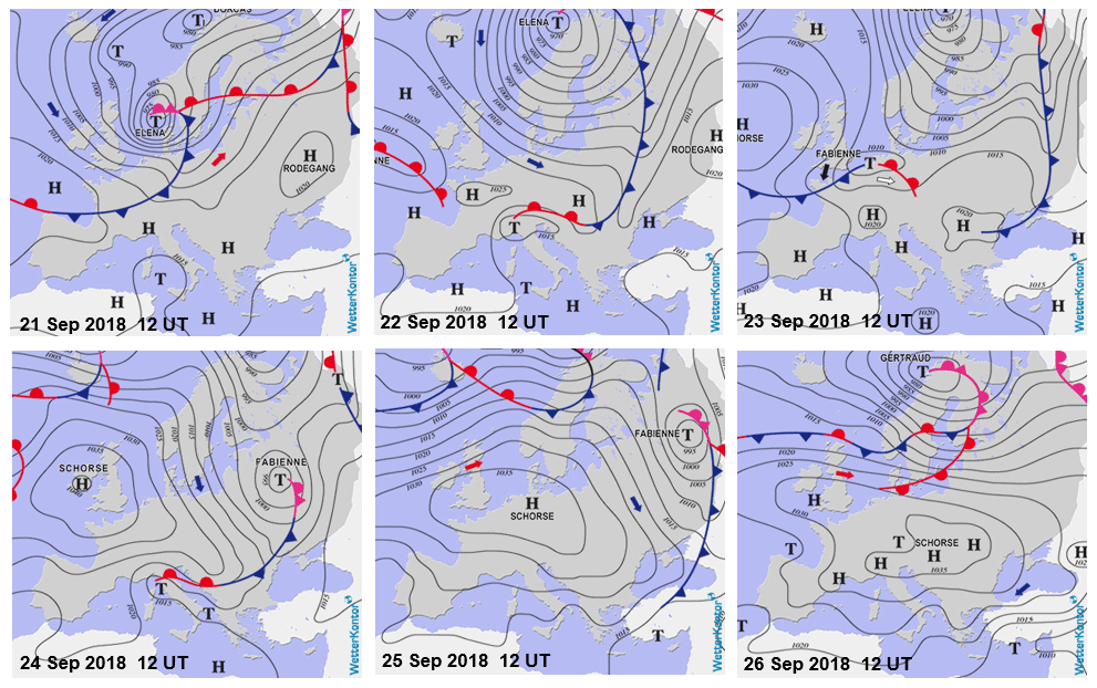
Figure 1Surface pressure maps provided by Wetterkontor, from https://www.wetterkontor.de, last access: 3 October 2018. Surface pressure is plotted with solid lines with 5 hPa steps. Atmospheric fronts (red curved lines with red semi-circles that point in the direction of the warm front, blue curved lines with blue triangles that point in the direction of the cold front and purple lines with alternating triangles and semi-circles pointing in the direction that the occluded front is moving) and the locations of the centers of high (H) and low (T) pressure systems are also presented.
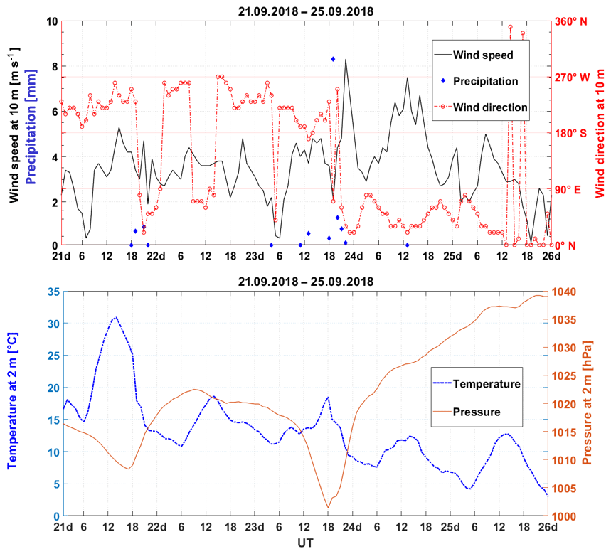
Figure 2Hourly average surface observations at the IAP meteorological station. Atmospheric pressure, air temperature and precipitation amount are measured at 2 m height above the surface, wind speed and direction at 10 m height above the surface.
Surface data: in Fig. 2, there are average hourly data measured at the Institute of Atmospheric Physics (IAP) meteorological station clearly showing the cold front that passed over this station at 18:00 UT on 21 September, when ground-level pressure reached a local minimum. Before the front, maximum air temperatures at 2 m reached tropical values above 30 ∘C; behind the front the maximum daily temperature did not reach more than 20 ∘C. The average hour wind speed intensified before the front and during the rainfall associated with storm activity. After passing the front, the surface wind changed from southwest to northeast.
Around 15:00 UT on 23 September, the warm front brought light rain associated with stratiform clouds. The temperature at 12:00 UT on 23 September was lower than in the afternoon, when the area was temporarily in the warm sector of cyclone Fabienne. The lifetime of the warm sector was very short. The time series of surface variables at the IAP station show the warm front which is connected with a slight directional wind shift but rapid rise in temperature until 18:00 UT on 23 September. At this time the passage of the cold front connected with Fabienne occurred and brought thunderstorm activity with heavy rain and wind shock. The surface pressure minimum was close to 1000 hPa, while the temperature reached the local maximum and the wind direction changed from west to north. The hourly mean wind speed rose rapidly up to midnight. On 24 September it was cold: the maximum temperature reached only 12.8 ∘C. The strong cold northwesterly wind remained across the measurement point, and the maximum averaged hourly values reached 7 m s−1 in the afternoon. Pressure continued to rise until midnight the following day. The center of the massive Shorse anticyclone (see Fig. 1), which moved from the British Isles over the Czech Republic in just 36 h, brought the pressure to a value of 1040 hPa.
Both the Europe surface pressure charts in Fig. 1 and the ground-level time series for the IAP observatory in Fig. 2 display an unusually fast passage of synoptic pressure patterns over central Europe. Cyclone Fabienne moved at around 25 m s−1. It exceeds speeds of extratropical transition. Jones et al. (2003) described extratropical transition of tropical cyclones which can accelerate from a forward speed of 5 m s−1 in the tropics to more than 20 m s−1 at the mid-latitudes. Sanders (1986) noted a mean surface cyclone speed moving at about 18 m s−1 for the cyclone that originated in the western-central North Atlantic and deepened explosively. A manual in the Czech language based on both empirical observations and classical synoptic meteorology states that the average cyclone speed over Europe is around 8 to 11 m s−1 (Kopáček and Bednář, 2009).
The synoptic-scale windstorm connected with cyclone Fabienne is an unusual event for the time of occurrence (23 September 2018) and for the storm moving velocity and intensity (Kašpar et al., 2017). The month of September in middle Europe is typically characterized by significant conditions under high pressure, i.e., relatively weak wind sunny days. Figure 3 exhibited the fast movement of cyclone Fabienne in a strong zonal flow from the Atlantic region across central Europe. Within the warm sector of the cyclone unstable wet air has been advected from the subtropical Atlantic region northeastward perpendicular to the direction of the cyclone movement. Follow-up strengthened baroclinity of the atmosphere at lower levels was the main cause of quick cyclone deepening (visible on surface pressure field – white lines) and generated storms at the head of the cold front.
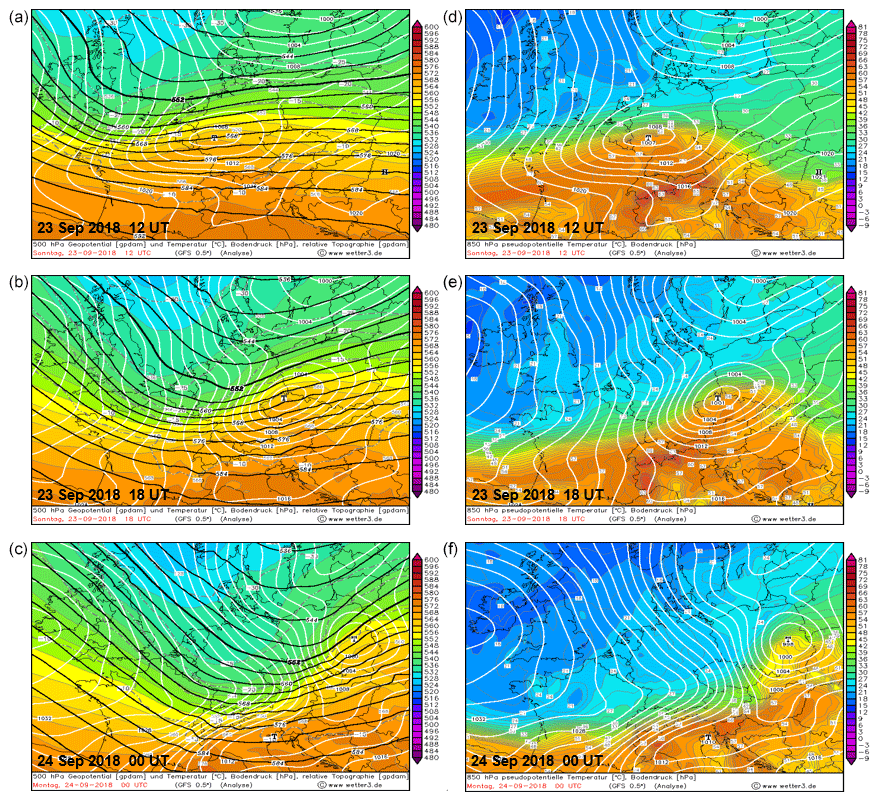
Figure 3(a) Distribution of the geopotential field (black lines) and temperature (gray dashed lines) at a level of 500 hPa, of the surface pressure field (white lines), and of relative topography 500–1000 hPa (color field). The 500 hPa is given in units of geopotential decameter (gpdam), the temperature in ∘C, the surface pressure in hPa, and the 500 / 1000 hPa thickness in gpdam. Isohypses and thickness are 4 gpdam apart, isobars 2 hPa and isotherms 5 ∘C. The thickness or difference in heights between the 1000 hPa (surface) and 500 hPa levels varies by temperature and moisture (is a function of the average virtual temperature); thus, the color field regions depicted the average temperature of the troposphere. (Orange/red values indicate warm tropical air, blue/indigo Arctic air.) (b) Analysis of pseudo-equivalent potential temperature in the 850 hPa pressure level in ∘C (color field and isotherms – gray lines, 3 ∘C apart) and surface pressure field (isobars – white lines, 2 hPa apart). The pseudo-equivalent potential temperature is conservative in association with the moisture; thus, it allows us to compare temperatures of air masses in the lower troposphere regardless of their humidity.
The 500 hPa map shows the main flow regime of the troposphere. (The atmosphere at an altitude about 5.5 km is no longer under the influence of surface friction. In synoptic meteorology a 500 hPa map is used to determine the speed and direction of synoptic patterns.) In the morning on 23 September the density of isohypses depicted at a 4 dam interval indicated a large pressure gradient between the warm southern and cold northern parts of Europe. At 12:00 UT the cyclone center is still located above Germany at 18:00 UT; it is above the territory of the Czech Republic. On the 850 hPa pseudo-equivalent potential maps there are clearly visible narrow transformation zones with a strong gradient of pseudo-equivalent potential temperature. These “warm boundaries” are separated various homogenous air masses with different temperatures and locate the position of the fronts on the surface pressure field (Kašpar, 2003). From radar images presented in Fig. 4, the speed of the squall line can be estimated at 110 km h−1. Impacts of the strong wind gusts associated with this squall line passage have been well documented in the European Severe Weather Database (https://www.eswd.eu, last access: 23 November 2018).
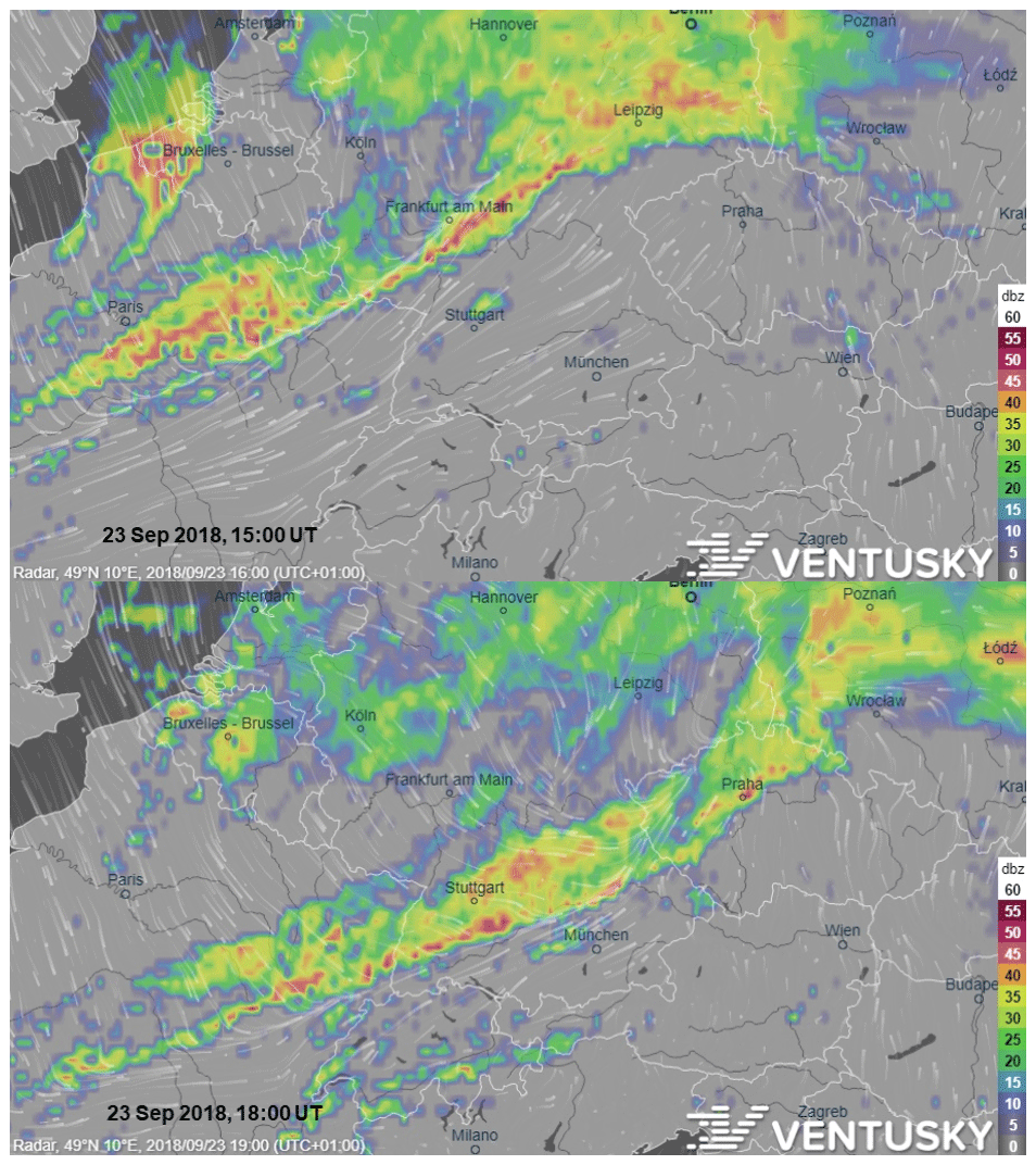
Figure 4Horizontal maximum projection of radar reflectivity from the European radar provided by VentuSky (https://www.ventusky.com, last access: 3 October 2018). There is a rapid shift of the strong thunderstorms' line (squall line) by 350 km per 3 h. White lines illustrate the wind speed at 10 m above the ground. The color scale indicates the radar reflectivity in 5 dBZ increments. The scale demonstrates the exponential dependence of the precipitation intensity (mm h−1) on radar reflectivity (dBZ). The value of 55 dBZ (dark purple) corresponds to the instantaneous value of the intensity of convective precipitation, 100 mm h−1.
Satellite Aeolus observation provides global wind profiles (along a single line-of-sight) up to an altitude of 30 km with an accuracy of 1 m s−1 in the planetary boundary layer (up to an altitude of 2 km). The Aeolus mission was launched on 22 August 2018 and scientific measurement started on 12 September 2018. All data outputs (including the ALADIN instrument) have already been verified and their reliability verified for the examined period. The Aeolus Earth Explorer Atmospheric Dynamics Mission yields data from global observations of wind profiles from space using the active DWL method (ESA, 1989; Durand et al., 2004). The DWL measurement is the unique method that provides data on a global scale from direct observation of wind. The Aeolus Doppler wind lidar measures 100 wind profiles per hour using both the Rayleigh and Mie scattering methods (for more information, see https://earth.esa.int/web/guest/missions/esa-operational-eo-missions/aeolus, last access: 10 December 2018).
The graphs in Fig. 5 display the wind profiles measured by the Aeolus ESA satellite using the ALADIN instrument working at 355 nm during the time period from 22 to 24 September 2018 (orbit numbers 481 to 520), geographical coordinate ranges: 12–19∘ E, 48–51∘ N, geomagnetic coordinates: 97∘ L, 48∘ F, −17∘ Y. The vertical axes represent altitudes of height bins, while the horizontal axes represent the time of observation. The data catalog is provided by ESA EO, from http://aeolus-ds.eo.esa.int/socat/L1B_L2_Products (last access: 7 January 2018). The accuracy is limited by the design of the instrument. In all the comparisons we consider this aspect. Single Doppler wind lidar is able to measure both Mie scattering from particles and aerosols and Rayleigh scattering from the upper atmosphere molecules. This study uses the Rayleigh scattering measurement with a random error (1σ) of 1 m s−1 at altitudes less than 2 km and 2 m s−1 between 2 and 16 km. Systematic error (1σ) is in this case smaller than 0.7 m s−1 (Durand et al., 2004).

Figure 5Aeolus Rayleigh scattering observations of wind profiles up to 20 km. The MDS wind profiles (positive towards the instrument) measured during orbit numbers 513 and 514 on 22–24 September 2018 between 04:32 and 06:51 UTC using the MDS Rayleigh scattering. The blue areas indicate zones during which the wind speed variations introduced by the Rayleigh response fluctuations are negative. Random error (1σ) is 1 m s−1 at altitudes less than 2 km and 2 m s−1 between 2 and 16 km. Systematic error (1σ) is smaller than 0.7 m s−1.
In the two upper panels of Fig. 5a and b we may see the situation before the storm on 22 September. At heights above 10 km there is an area where the satellite registers the opposite direction of the wind compared to the surrounding regions (marked by blue color). Figure 5c represents the situation of the early morning of 23 September before cyclone Fabienne has entered the area of the measurement site. Calming of the wind flow caused by the temperature daily cycle is clearly visible. Figure 5d shows the post-storm effect on 24 September. The area of the opposite wind direction detected by satellite Rayleigh scattering is lifted up to heights of 15 km. The measurements at the time of the Fabienne storm passage above the measurement site are not available due to the satellite trajectory; however, from the satellite records before and after, the cyclone passage indicates extremely high speed changes within the troposphere and lower stratosphere.
The stratosphere and its dynamics are very sensitive to wave activity in the higher or lower layers (troposphere or mesosphere). That is why the strong storm Fabienne as a source of many different kinds of waves should bring disturbance into regular dynamics. With changes in dynamics are connected changes in temperature and vice versa. Stratospheric wind and temperature for the European region are presented for the time span 20 September at 00:00 UT to 27 September at 18:00 UT (each day is represented by one row in the figures). This period covers a whole week (3 d before and 4 d after the Fabienne storm).
Figure 6a shows zonal wind at 1 hPa for the European region from 20 September at 00:00 UT to 27 September at 18:00 UT. In the sequence there is a well-seen weak eastward wind in middle Europe and westward wind in southern Europe, which is a typical situation for this period. Shortly before storm Fabienne (23 September 00:00 and 06:00 UT) easterly wind became stronger and replaced westerly wind in the south (because of incoming waves from the troposphere) and remained easterly for the following several days in the whole of the studied area. At 0.1 hPa we can see changes from westerly to easterly wind shortly after Fabienne (24 September 00:00 and 06:00 UT). We do not register any significant changes before because waves from the troposphere need some time to reach 0.1 hPa. Strong easterly wind remains in the whole of Europe again for several days after the storm. The stratosphere needs some time to change/restore dynamics to normal situations because of wave disturbances which remain in the inversion condition (temperature increase with altitude) much longer than in other layers. That is why we can observe strong eastward wind not only during the storm, but also for several days after the storm in the whole of Europe as well.

Figure 6Stratospheric wind above Europe at 1 hPa (a) and at 0.1 hPa (b). Red color represents eastward wind, and blue represents westward wind.
The changes in the zonal wind, which mainly control stratospheric dynamics (meridional wind is much weaker but very important for Dobson–Brewer circulation), are usually connected with changes in temperature because strong zonal wind effectively blocks air mixing form different latitudes, especially at higher latitudes. The temperature is observed directly, so we can expect better approximation in reanalysis than for zonal wind, which is the derived parameter. The temperature fields at 1 hPa are presented in Fig. 7a. We can find much colder air in middle and northern Europe shortly before and mainly after storm Fabienne (23 September 06:00 and 12:00 UT) because usually strong barriers (different winds between high and lower latitudes) are destroyed after Fabienne and much colder air from the polar vortex can reach lower latitudes, in our case middle and southern Europe. Colder air at lower latitudes for several days after storm Fabienne could impact not only the chemistry in the higher stratosphere in autumn, but mesosphere conditions as well (i.e., the propagation of waves could be slower or faster than usual or they can be absorbed into the stratosphere). This change is well connected with change in zonal wind.
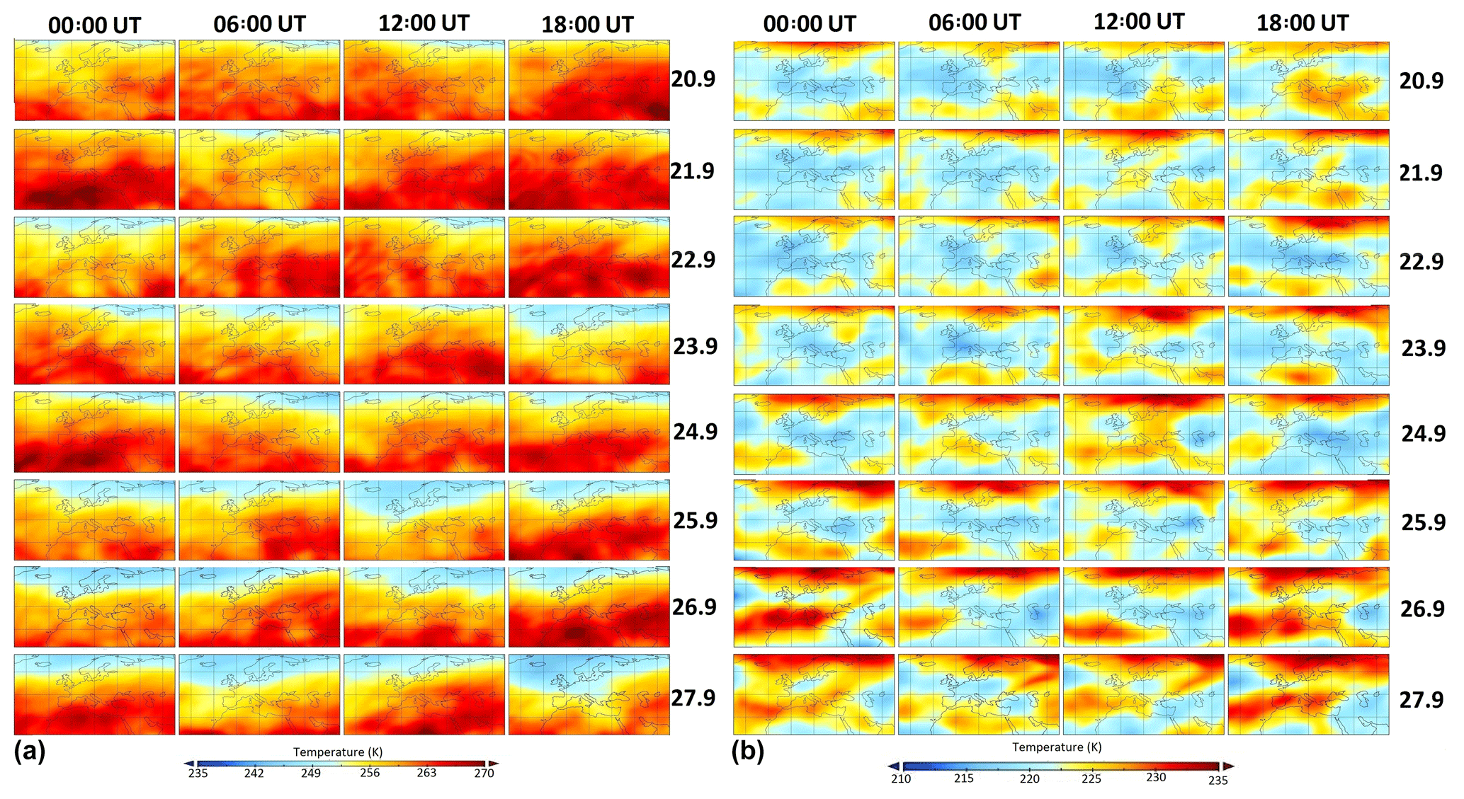
Figure 7Stratospheric temperature above Europe at 1 hPa (a; temperature in the range 235–270 K) and at 0.1 hPa (b; temperature in the range 210–235 K).
At 0.1 hPa (in Fig. 6b) the change in the zonal wind is even stronger than at 1 hPa (compare Fig. 6a and b) because the wind in the mesosphere is usually stronger than in the stratosphere. As was indicated in the wind results, several hours after the storm (24 September 06:00 and 12:00 UT) zonal wind changes from westward or very weak eastward to strong eastward and remains without changes for several days. Meridional wind in the mesosphere is stronger than in the stratosphere, but zonal wind still plays a major role in the dynamics changes. Temperature changes at this level, which corresponds to the lower mesosphere, are opposite from pressure level 1 hPa. There is warmer air at higher latitudes, so stronger eastward wind brings this warmer air to the lower latitudes (because it is not blocked by the westward wind) and affects the whole area of middle Europe. The warmer air stays in the analyzed area because we need to wait until the zonal wind reverses to its usual state (westward instead of eastward). We have to notice that 0.1 hPa is above the stratosphere, and the dynamics here could be affected by different processes (solar radiation, chemistry, etc.) than at 1 hPa (almost the stratopause).
Especially 0.1 hPa is on the top of the MERRA-2 reanalysis, so we should be very careful with interpretation of the results, because the information from this level could be affected by a border condition or problem with wave activity dissipation. But we need mainly qualitative description rather than quantitative description for our study, so information from MERRA-2 is sufficient.
September 2018 was a period of rather low geomagnetic activity. On 4 September the geomagnetic activity increased for about 20 h. The maximum registered Kp index was Kp = 6. The following period was characterized by low geomagnetic activity with Kp up to 3 till 18 September, when the Kp index fell down to 0 and remained very low till 21 September. On 21 September the geomagnetic activity increased again at 22:30 UT when Kp = 4+. Increased geomagnetic activity lasted for about 20 h with a maximum Kp = 5− on 23 September at 03:00 UT. The activity can be classified as a minor to moderate geomagnetic storm. On 23 September, the geomagnetic activity fell again to values around Kp = 2 to 2+. In general, there was rather low geomagnetic activity with only short slightly enhanced events. However, the geomagnetic effects are responsible for part of the observed ionospheric variability and cannot be completely neglected. Geomagnetic indices were downloaded from Potsdam Data Center (https://www.gfz-potsdam.de/en/kp-index/, last access: 21 November 2018). A detailed plot of the geomagnetic Kp index for the time span 21–26 September is provided as a part of Fig. 10c.
An example of multi-beam ionograms measured by DPS-4D is shown in Fig. 8. There is a sequence of ionograms recorded during 4 consecutive days around 23:00 UT. The receiving antenna system of the digisonde is able to identify the direction of the electromagnetic wave arrival. The information about the reflected wave arrival is included in the raw ionograms. Further, from the sequence of raw ionograms the general plasma motion is constructed and presented as the directogram. Each color corresponds to a particular antenna beam, hence the direction of the arrival of an oblique echo from large-scale irregularities. Colors of the echo indicate a particular direction of arrival. It is clearly shown that the echo changes significantly. The ionogram at 23:00 UT is selected to show the changing dynamics of the ionospheric plasma. During night time, ionograms with a clear echo are typically recorded. The antenna system registers practically only a vertically reflected signal, as is shown in panel (a) measured on 22 September and panel (d) recorded on 25 September. In comparison, a qualitatively different pattern is detected in panels (b) and (c). The echo in panel (b), recorded on 23 September shortly after the passage of the cold front with heavy storm activity, is called the spread F situation. As is indicated by the color scheme on the right-hand side of each ionogram, the antenna system records echoes from practically all sounding beams. Both vertical and off-vertical echoes are spread in height and frequency. This means that the ionosphere is full of irregularities and iso-contours of electron concentration are significantly undulated. In panel (c) measured on 24 September, there is a well-recorded vertical echo and slightly higher oblique structure reflected from the north-northeasterly direction. Such kinds of echoes are known as spur echoes and may appear when ionospheric iso-contours are significantly tilted. In general, the vertical echo in panel (c) corresponds to the situations in panels (a) and (d). The spread F situation in panel (b) indicates significant wave-like activity within ionospheric plasma in the F region.
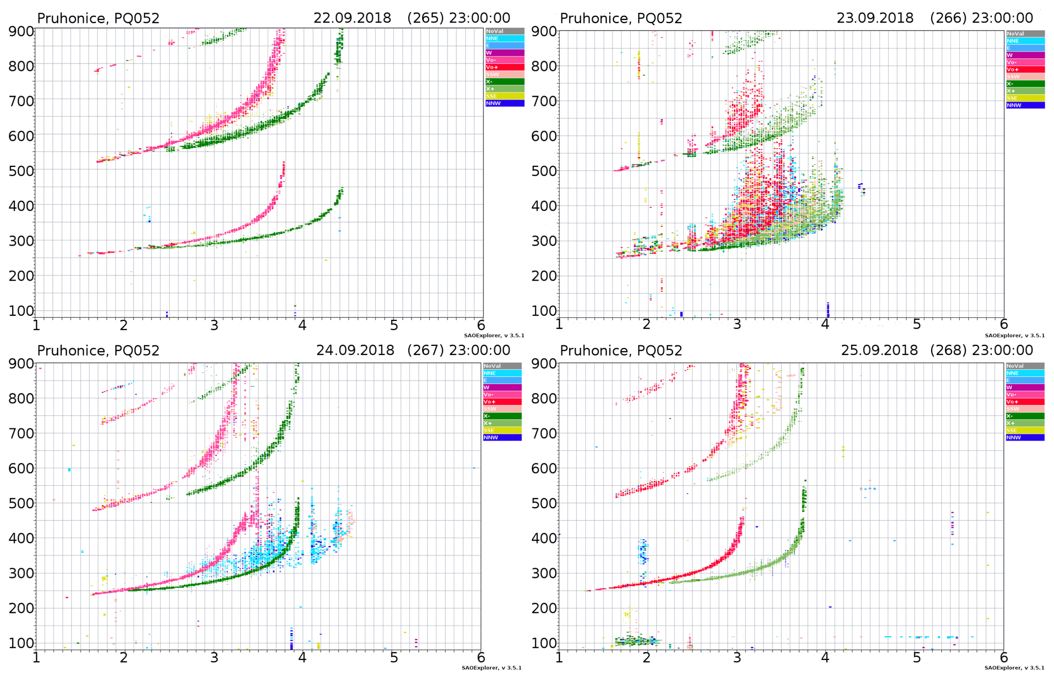
Figure 8Sequence of ionograms recorded during local night at around 23:00 UT presented in a standard DPS-4D format. A particular color indicates the direction of radio wave arrival. The vertical echo of an ordinary wave is marked by red color, while green color stands for an extraordinary wave. Other colors represent non-vertical reflections. The strongest non-vertical echo comes from the north-northeasterly direction (light blue color).
A sequence of directogram measurements recorded by DPS-4D is shown in Fig. 9. There are two distinct episodes of increased activity. On the directograms measured on the first two days, 21–22 September, wave activity is rather low. The situation changes significantly on 23 September at 17:00 UT, when a strong echo is recorded till 24 September at 04:00 UT. The signal detected by the receiver varies significantly during the night. An interesting fact is that the DPS-4D instrument detects strong quickly changing plasma shears and reversal plasma motion with respect to the zero zenith angle. There is no prevailing or characteristic plasma flow for the event. During day time, there is very low activity visible on the directogram till the evening hours. A strong echo is recorded again from 24 September at 17:00 UT till 25 September at 04:00 UT. However, the echo is not as strong as the preceding night with smaller shears. Prevailing or dominant plasma motion during the local night of 24–25 September is in the north-northeasterly direction.
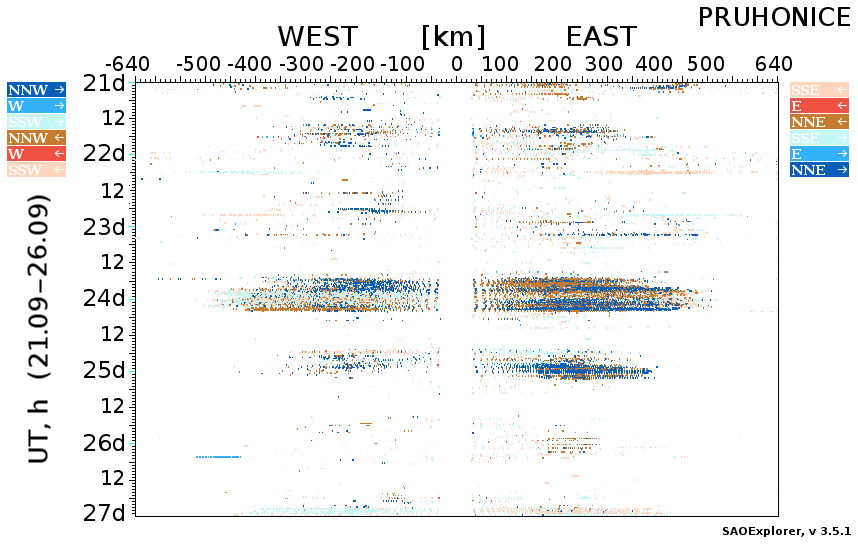
Figure 9Directogram – direction of plasma motion above the observation site – recorded on 21–26 September presented in a standard DPS-4D format. Due to the geometry of the receiving antenna field, DPS-4D identifies the direction of the wave arrival. The directograms are constructed from the raw ionograms. Each color corresponds to a particular antenna beam, hence the direction of the arrival of an oblique echo from large-scale irregularities. It is denoted by a particular color on the left- and right-hand sides of the diagram.
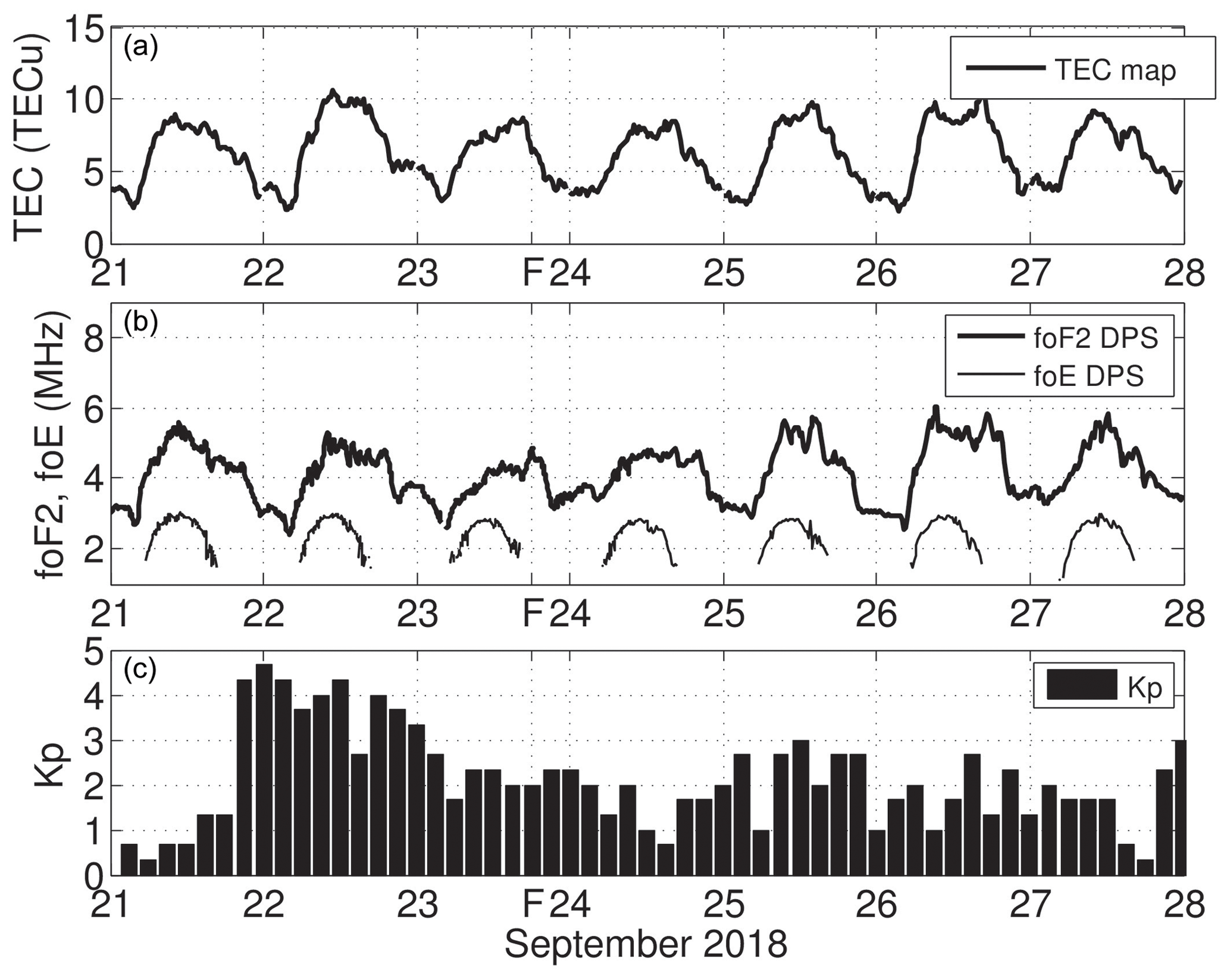
Figure 10Diurnal courses of total electron content (a), critical frequencies foF2 and foE (b) above station Pruhonice (“F” denotes the time of passage of storm Fabienne over the station) and the course of the Kp index (c) during the observational period.
In the plot of the diurnal course of TEC in Fig. 10a, a decrease can be observed on 23–24 September compared to the previous day, 22 September. Similarly in Fig. 10b, a decrease in critical frequency foF2 was observed during 23–24 September. While TEC and foF2 show a significant decrease in reaction to minor geomagnetic disturbance, there is no clear change in the course and shape of the critical frequency of E layer foE (Fig. 10b) except for very short wave-like variability on 23 September before the Fabienne storm passage above the observational site. On 23 September, the maximum of foE reaches the same values as on the preceding and following days. Most of the variability is observable within time series of TEC and foF2, and both parameters agree well through the studied interval. Their matching can be explained by a dominant contribution of the F2 layer's electron content contribution to the TEC and a much lower contribution of the E layer's variability during the studied days, even during the Fabienne event. The effect of electron concentration decrease on the ionosphere can be attributed to the geomagnetic disturbance observed as a negative storm effect (Prölss, 2004) related to the decrease in the atomic oxygen leading to a decrease in production of oxygen ions and the increase in molecular nitrogen density leading to the increase in the loss rate of ion species. Both processes lead to electron–ion concentration decrease. Values of critical frequencies foF2 and TEC return to typical values of the season comparable with those preceding the observed geomagnetic storm event on 25 September (2 d after the storm passage over Pruhonice station). Geomagnetic disturbance started on 21 September at 21:00 UT. Frequency foF2 during night falls much faster than is typical. Then during the night of 22–23 September, critical frequency foF2 falls even faster, oscillates and remains below 3.5 MHz till almost noon, when it rapidly increases. During the night of 23–24 September, after sunset critical frequency foF2 decreases faster compared to the nights of 21–22 September and 25–26 September, when a typical course of foF2 is registered.
The observed variability of the parameters TEC, foF2 and foE in Fig. 10 is caused jointly by the minor geomagnetic disturbance and atmospheric waves associated with the Fabienne storm. It is practically impossible to distinguish which part of the variability belongs to the particular forcing. Ionospheric vertical sounding has, unfortunately, limitations and provides integral information about the resulting behavior of the atmosphere. However, in addition to the time of flight of the electromagnetic wave the DPS-4D equipment recorded additional parameters of the reflected wave from the ionosphere. Variability of critical frequency foF2 must be interpreted together with the complete ionogram record. As is demonstrated in Fig. 8, there is a well-seen change in the ionogram pattern through experiment. Ionograms recorded on 22 September (type in panel a) are usually recorded when the reflection plane is practically flat, while ionograms recorded on 23 September (type in panel b) are measured when reflection planes are significantly undulated. Such situations occur in association with atmospheric wave activity. Hence, this additional information can be used to slightly untangle effects of the geomagnetic disturbance and convective activity. Taking into account the course of foF2 and TEC together with a change in ionogram reflection patterns, we suppose that the dominant effect of the geomagnetic disturbance is pronounced as a decrease in foF2 and TEC, while short-term wave-like variability around the mean course associated with spread echo occurrence on ionograms can be attributed to the convective activity in the lower atmosphere.
All ionograms were manually scaled and further used for determination of the vertical profile of electron concentration (or frequency) with the use of the NHPC inversion technique that is part of the Digisonde software. Details and downloads are available on the web page: http://umlcar.uml.edu/digisonde.html, last access: 26 November 2018. In agreement with the course of foF2 and TEC, analyses of entire electron density profiles reveal the same decrease on 23–24 September as a consequence of the preceding geomagnetic moderate storm. In order to illustrate well the electron concentration variability related to the cold front effect, we focus on profilograms for 3 consequent days: 22–24 September.
Due to geomagnetic disturbance electron concentration, the corresponding plasma frequency decrease leads to problematic representation of the situation for the entire time span of 21–26 September. Figure 11 shows variations of the reflection height of the sounding signal recorded on 22–24 September for the selected range 2–6 MHz with a 0.1 MHz step. Oscillations in heights clearly show strong wave-like activity within all ionospheric heights. Comparing reflection heights at fixed frequencies for two consecutive nights, there are shorter period oscillations visible during the night on 22–23 September compared to the night time on 23–24 September. Oscillations detected during both nights are coherent through all levels.
Similar effects of oscillation to those observed in Fig. 11 are seen in the detailed plot of profilograms in Fig. 12 composed of true-height profiles during all the analyzed days. Deviation from the regular course is clearly seen in the profile thickness that is significantly smaller on 23 September till 24 September at about 06:00 UT, when the thickness of the profiles increases again.
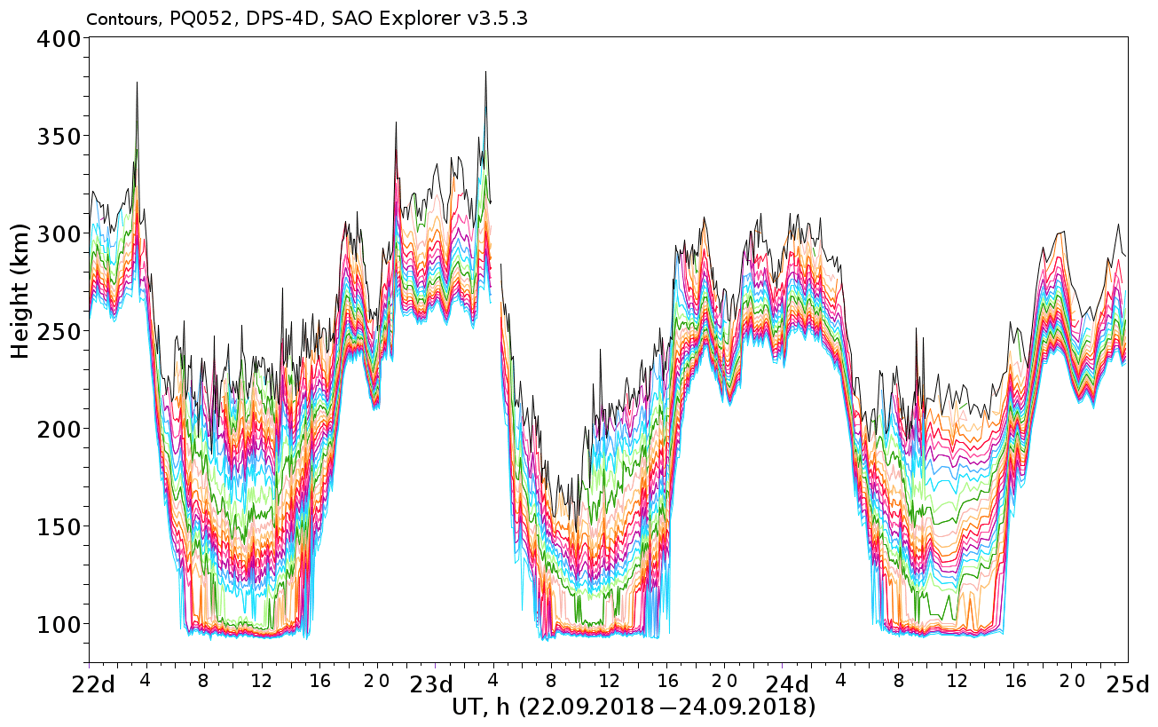
Figure 11Variability of true-height reflection at fixed frequencies recorded during 22–24 September for the frequency range 2–6 MHz with a 0.1 MHz step, in a standard DPS-4D format.
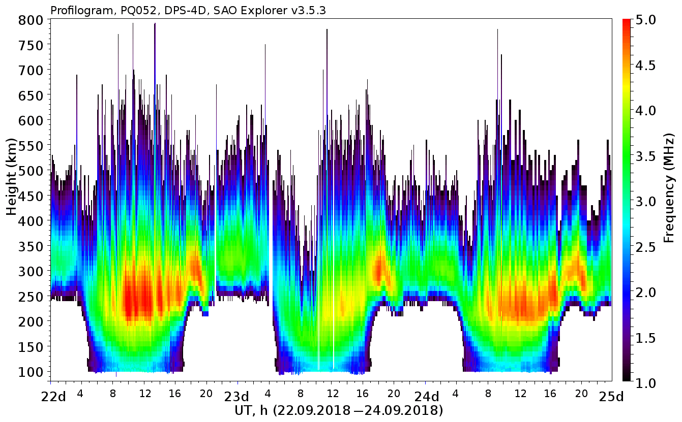
Figure 12Detail of profilograms in frequency – 22–24 September presented in an a standard DPS-4D format.
Further we have analyzed critical frequency foF2 using continuous wavelet transform to obtain the power content in particular periods. The wavelet power spectrum (WPS) for 21–26 September is presented in Fig. 13. Oscillations on shorter periods on 22 September compared to 23 September are seen well in Fig. 13. In the plot of the WPS, there are high power domains of short-period oscillation in the range 5–30 min during day time on 21 and 22 September. Less energy is detected during day time on 23 September. Missing spectral content in periods below 30 min on 24–26 September is caused by a change in the sounding rate on 24 September at 10:00 UT. As has been explained in the data section, a high sampling rate campaign was switched till morning on 24 September for study of a sporadic-E phenomenon.
The following three panels in Fig. 14 show the ionospheric drift evolution on 20–27 September. In the plots of the northern (panel b) and eastern (panel c) components, during several days preceding both geomagnetic and meteorological storm there are only rare situations where the ionospheric plasma motion was detected in a horizontal plane. An episode of longer duration of plasma flow in the horizontal plane is detected after sunset on 23 September when storm Fabienne hit the observation point. The characteristic value of plasma flow velocity is vNorth∼40 and m s−1. Comparing the northern component of the plasma flow during the night of the Fabienne storm (24 September at 01:00–04:00 UT) and the corresponding time on the following days, it is important to point out that the flow is in the opposite direction and practically the same velocity magnitude.
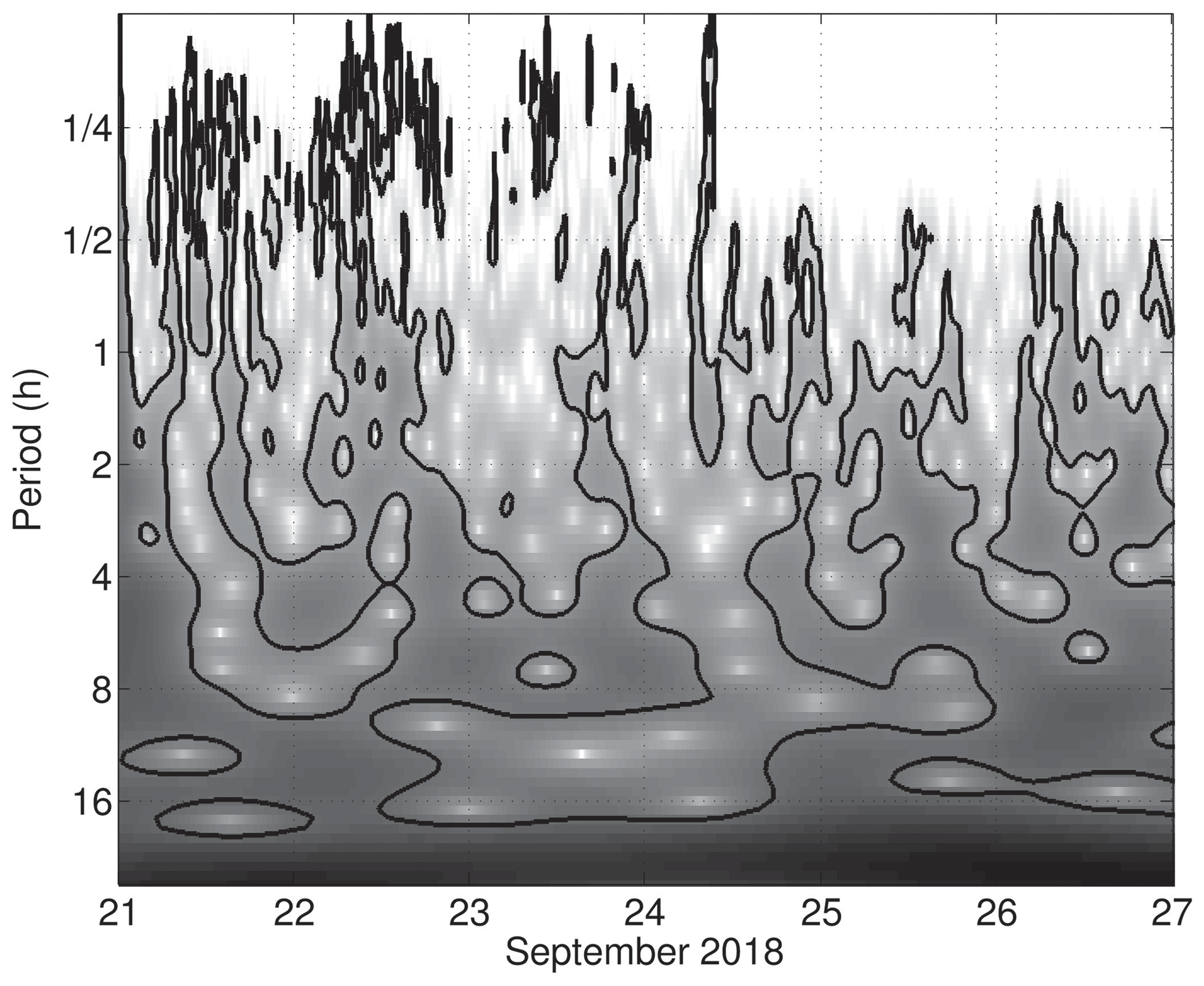
Figure 13Wavelet power spectra of critical frequency foF2 for 21–27 September 2018. WPS is normalized on each scale to the corresponding scale maximum. Dark areas exceed the 0.95 significance level on each scale.
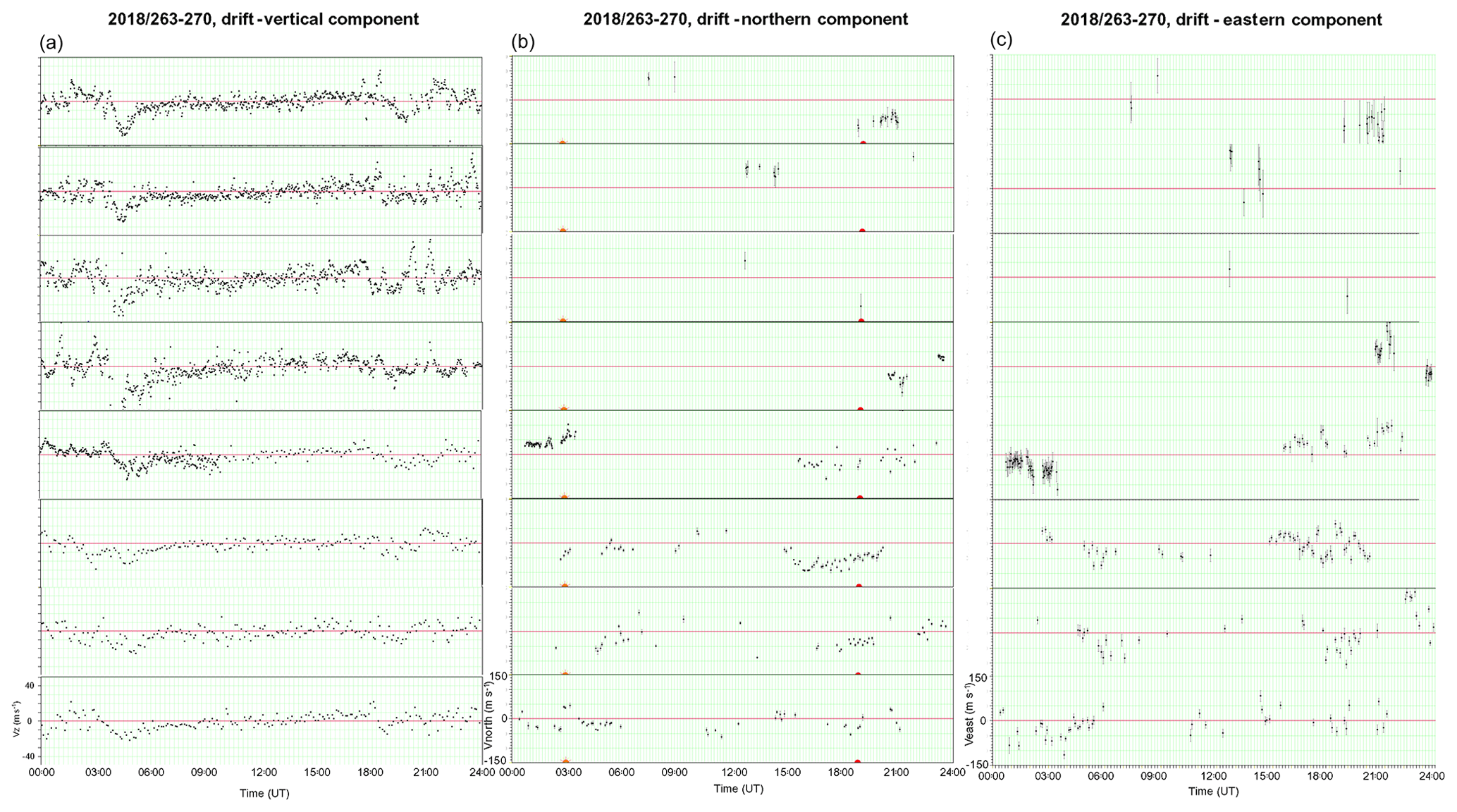
Figure 14Components of ionospheric plasma drift obtained by Digisonde DPS-4D during the studied event on 20 September (top panel) to 27 September (bottom panel) – (a) vertical component; (b) northern component; (c) eastern component presented in a standard DPS-4D format.
Vertical components in Fig. 14a show a typical diurnal course with two minima, one located close to sunrise and one close to sunset (same as that reported by Kouba and Koucká Knížová, 2016). Values of the vertical drift before the Fabienne storm event reached regularly larger values with respect to days after the event. For instance, magnitudes of sunrise negative velocity peaks are detected around to −30 m s−1, while after the event sunrise peaks do not exceed m s−1. The abrupt change is seen on 23 September at 19:00 UT, soon after the cold front passing above the observation point. Characteristic values before the storm exceed vv∼20 m s−1, while after the storm they hardly reach vv∼20 m s−1 and rather stay close to vv∼10 m s−1. Change in plasma flow is well pronounced in all three drift velocity components shortly after the frontal passage above the observational point at ground level.
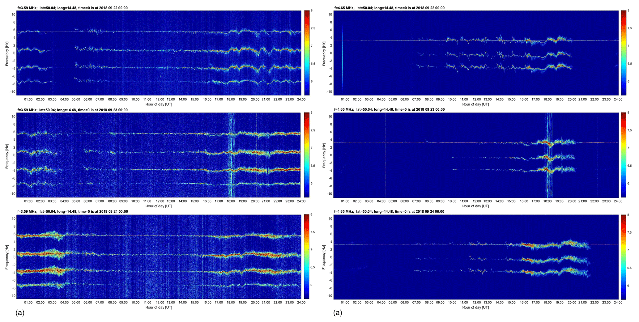
Figure 15Continuous Doppler sounding measurement on 3 consequent days 22–24 September at frequencies 3.59 (a) and 4.65 MHz (b).
In the following Fig. 15, we show CDS measurement on 3 consequent days 22–24 September at frequencies 3.59 (a) and 4.65 MHz (b). The beginning of storm Fabienne (or the passage above the observational point) is visible in the data as a short-duration increase in noise across the CDS spectra at both frequencies. Qualitative change in the echo is evident for the first sight. Data were obtained from continuous Doppler sounding spectrogram archive IAP CAS, Prague, http://datacenter.ufa.cas.cz/, last access: 22 October 2018. Spectrograms of the recorded infrasound during event Fabienne until 04:00 UT correspond to the reference time for this event.
The spectral content changed with time and was different during the strong storm event compared to the preceding and following days. During the afternoon hours on 22 September, CDS registers a clear sharp echo with wave-like fluctuations. On 23 September at both frequencies we have observed a sudden increase in noise at 18:00 UT that could indicate the arrival of an acoustic wave packet from the frontal border. After that, a stronger and blurred echo compared to 22 September is registered at both frequencies. Wave-like fluctuations are not detected within the signal at 3.59 and 4.65 MHz. At both frequencies (better pronounced at 4.65 MHz in Fig. 15b), there are apparent coincidental drops in frequency at 18:00 UT. A blurred strong echo was observed until around 04:00 UT on 24 September. In the afternoon hours on 24 September, the recorded CDS echo remains slightly blurred, but it is significantly weaker. The occurrence of a stronger echo on CDS sounding at 3.59 MHz in the interval 18:00 UT (23 September) till 04:00 UT (22 September) corresponds to the increased wave activity on directograms and detection of plasma flow on both northern and eastern plasma drift components. The trace of 4.65 MHz is limited due to the diurnal course of foF2. Hence the changes in the CDS signal can be discussed only till 20:00 UT. The signal detected on 23 September is significantly stronger with respect to the preceding and following days, especially in the part that corresponds to the frequency drop at 18:00 UT.
According to our experience in Chum et al. (2018), we can conclude that we observe disturbances related to waves propagating from a lower-laying atmosphere. It was shown that the co-typhoon infrasound waves were recorded in the spectral range from ∼3.5 to 20 mHz with a maximum of spectral density around 5 mHz (dominant periods between 3 and 4 min). The spectra revealed fine structures that were likely caused by modal resonances.
We have analyzed atmospheric and ionospheric effects induced by the fast transit of a cold front with a strong storm of cyclone Fabienne. The cold front passed above Europe within 24 h with high speed, reaching a value of 30 m s−1 (approx. 108 km h−1) on 23 September 2018. The synoptic-scale windstorm connected with cyclone Fabienne was atypical in its time of occurrence, and the velocity of the storm moving activity highly exceeded standard values for the season. The temperature drop on the frontal border of 10 ∘C is also rather large. The major damages were caused by the storms on the frontal border mainly on the territory of Germany, where the wind gusts reached an extreme value of 45 m s−1 (162 km h−1). In the Czech Republic, the strongest wind gusts of about 35 m s−1 (126 km h−1) were recorded in the mountains. Significant strong wind was observed in the lowlands as well. For instance, in meteo-station Karlov, located in Prague, wind gust reached a value of 27 m s−1 (97 km h−1).
We have detected a significant change in the dynamical pattern in the stratosphere following immediately after the storm in both wind and temperature. The general circulation pattern above Europe at 0.1 hPa before the storm Fabienne event can be classified/characterized as part of the stratosphere in normal conditions in September. Based on that, we attribute the overall change in the stratospheric circulation/dynamics to the strong wave field that was launched upward from the fast-moving mesoscale system.
At the time of the Fabienne event, the ionosphere was slightly influenced by a minor to moderate geomagnetic storm that occurred 1 d before. According to the evolution of the Kp index and ionospheric plasma parameters (TEC and foF2), the ionosphere was already in the recovery phase of the geomagnetic storm. Nevertheless, the observed disturbances are induced by both geomagnetic storms and convective activity in the lower-laying atmosphere. Regarding the results of the model study (Pedatella and Liu, 2018), we attribute a general decrease in foF2 and TEC to the geomagnetic forcing (longer-term, negative storm scenario) and a significant increase in wave-like activity (short-term, wave-like activity) to the convective system forcing.
We have found significant departures from typical values of ionospheric parameters shortly after the transition of the cold front across the observation point. We have detected a sudden strong increase in wave-like activity on the directograms and CDS records. The detected strong echo on directograms shows strong and rapid changes in the horizontal plasma motion. During the observation, there was no prevailing plasma motion direction. It rather accounts for turbulent flow within the F layer. In the strong echo in directograms attributed to the storm, there is no characteristic prevailing motion, but sudden changes in direction are observed through the event. Time-limited increase in plasma drift in the northerly and easterly directions has been detected together with a decrease in velocity of the vertical plasma flow. Wave-like oscillations are present within ionospheric plasma all the time. In the WPS spectra of critical frequency we have detected a change in the spectral content during the day of the Fabienne event compared to the preceding day. We have noticed a decrease in the F-layer thickness during the day of the Fabienne event. Irregular stratification of the ionosphere is confirmed by a spread echo recorded by Digisonde during the afternoon and night on 23 September till the morning of 24 September. CDS data show a significant change in the spectral content, shape and power of the registered signal, corresponding to modulation by waves propagating from the convective system.
From the results summarized above we conclude that mesoscale systems are effective sources of atmospheric disturbances that can reach ionospheric heights and significantly alter atmospheric and ionospheric conditions. Convective system Fabienne affected Earth's atmosphere on a continental scale and up to F-layer heights. Even during periods of geomagnetic disturbance and minor to moderate geomagnetic storms, the contribution of the lower atmosphere to the ionospheric dynamics cannot be neglected. Our experimental result is in agreement with the theoretical study of Pedatella and Liu (2018) that internal atmosphere variability should be taken into account even during geomagnetic disturbances.
We have used code for scaling and evaluation of ionospheric data measured by DPS-4D. The code was developed in the Space Science Lab, at the University of Massachusetts Lowell. The code and its regular upgrades are available for public at the university page: http://umlcar.uml.edu/digisonde.html, last access: 5 September 2018.
All the data used for the research are available for the public. They can be downloaded via the following sites. Meteorological ground-based data comprise meteoradar reflectivity (https://www.ventusky.com/, last access: 3 October 2018), surface pressure maps (https://www.wetterkontor.de/, last access: 3 October 2018), geopotential field and temperature at a level of 500 hPa, and pseudo-equivalent potential temperature in the 850 hPa pressure level (http://wetter3.de, last access: 3 October 2018), surface observations at the IAP meteorological station (http://www.ufa.cas.cz/institute-structure/department-of-meteorology/present-weather-sporilov.html, last access: 3 October 2018), and Aeolus Rayleigh scattering wind profiles (http://aeolus-ds.eo.esa.int/socat/L1B_L2_Products, last access: 10 December 2018). Stratospheric wind and temperature reanalysis MERRA-2 data can be downloaded from https://disc.gsfc.nasa.gov/daac-bin/FTPSubset2.pl, last access: 15 November 2018. Ionospheric ground-based data involve DPS-4D measurements (http://digisonda.ufa.cas.cz/, http://giro.uml.edu/, last access: 26 November 2018) and continuous Doppler sounding spectrograms (http://datacenter.ufa.cas.cz/, last access: 22 October 2018). Total electron content maps can be found on http://gnss.be/Atmospheric_Maps/ionospheric_maps.php, last access: 10 October 2018. The geomagnetic Kp index is available on https://www.gfz-potsdam.de/en/kp-index/, last access: 21 November 2018.
PKK did the DPS-4D ionogram data scaling, analyses and interpretation, and wrote the first draft of the paper. KAPO did AEOLUS data analyses and interpretation, CDS data analyses and interpretation. KACA did meteorology data preparation and interpretation. DK did DPS-4D settings and drift data analyses. ZM did TEC data analyses and interpretation and figure preparation. JB did DPS-4D data interpretation. MK did stratospheric data analyses and interpretation.
Petra Koucká Knížová is one of the special issue editors of Annales Geophysicae.
This article is part of the special issue “Vertical coupling in the atmosphere-ionosphere system”. It is a result of the 7th Vertical Coupling workshop, Potsdam, Germany, 2–6 July 2018.
The authors would like to thank colleagues from the Institute of Atmospheric Physics (CAS), Marek Kašpar for synoptic interpretation of Fabienne cyclone peculiarities, and furthermore Jaroslav Chum, Jiří Baše and František Hruška for maintenance of the Doppler systems. The authors would like to acknowledge the Global Ionosphere Radio Observatory (GIRO) and its mirror site hosted in the Institute of Atmospheric Physics (CAS).
The work of Petra Koucká Knížová, Daniel Kouba, Zbyšek Mošna, and Josef Boška was supported by the Research Executive Agency (H2020-COMPET-2017, TechTIDE – grant no. 776011). The work of Kateřina Podolská was supported by the Czech Science Foundation (grant no. 18-01969S) and the work of Michal Kozubek by the Czech Science Foundation (grant no. 18-01625S).
This paper was edited by Erdal Yiğit and reviewed by two anonymous referees.
Afraimovich, E. L., Astafyeva, E. I., Demyanov, V. V., Edemskiy, I. K., Gavrilyuk, N. S., Ishin, A. B., Kosogorov, E. A., Leonovich, L. A., Lesyuta, A. S., Palamartchouk, K. S., Perevalova, N. P., Polyakova, A. S., Smolkov, G. Y., Voeykov, S. V., Yasyukevich, Y. V., and Zhivetiev, I. V.: A review of GPS/GLONASS studies of the ionospheric response to natural and anthropogenic processes and phenomena, J. Space Weather Space Clim., 3, 19 pp., https://doi.org/10.1051/swsc/2013049, 2013.
Alexander, M. J., Holton, J. R., and Durran, D. R.: The Gravity Wave Response above Deep Convection in a Small Line Simulation, J. Atmos. Sci., 52, 2212–2226, 1994.
Anthes, R. A.: Exploring Earth's atmosphere with radio occultation: contributions to weather, climate and space weather, Atmos. Meas. Tech., 4, 1077–1103, https://doi.org/10.5194/amt-4-1077-2011, 2011.
Azeem, I., Yue, J., Hoffmann, L., Miller, S. D., Straka III, W. C., and Crowley, G.: Multisensor profiling of a concentric gravity wave event propagating from the troposphere to the ionosphere, Geophys. Res. Lett., 42, 7874–7880, https://doi.org/10.1002/2015GL065903, 2015.
Barta, V., Haldoupis, C., Satori, G., Buresova, D., Chum, J., Pozoga, M., Berenyi, K. A., Bor, J., Popek, M., Kis, A., and Bencze, P.: Searching for effects caused by thunderstorms in midlatitude sporadic E layers, J. Atmos. Sol.-Terr. Phys., 161, 150–159, 2017.
Bhar, J. N. and Syam, P.: Effects of thunderstorms and magnetic storms on the ionization of the Kenelley-Heaviside Layer, Phil. Mag. J. Sci., 23, 513–528, https://doi.org/10.1080/14786443708561823, 1937.
Boška, J. and Šauli, P.: Observations of gravity waves of meteorological origin in the F-region, Phys. Chem. Earth Pt. C, 26, 425–428, 2001.
Buonsanto, M. J.: Ionospheric storms – A review, Space Sci. Rev., 88, 563–601, 1999.
Chernigovskaya, M. A., Shpynev, B. G., and Ratovsky, K. G.: Meteorological effects of ionospheric disturbances from vertical radio sounding data, J. Atmos. Sol.-Terr. Phys., 136, 235–243, https://doi.org/10.1016/j.jastp.2015.07.006, 2015.
Chernigovskaya, M. A., Shpynev, B. G., Ratovsky, K. G., Belinskaya, A. Yu., Stepanov, A. E., Bychkov, V. V., Grigorieva, S. A., Panchenko, V. A., Korenkova, N. A., and Mielich, J.: Ionospheric response to winter stratosphere/lower mesosphere jet stream in the Northern Hemisphere as derived from vertical radio sounding data, J. Atmos. Sol.-Terr. Phys., 180, 126–136, https://doi.org/10.1016/j.jastp.2017.08.033, 2018.
Chum, J., Liu, J.-Y., Podolská, K., and Šindelářová, T.: Infrasound in the ionosphere from earthquakes and typhoons, J. Atmos. Sol.-Terr. Phys., 171, 72–82, 2018.
Clilverd, M. A., Ulich, T., and Jarvis, M. J.: Residual solar cycle influence on trends in ionospheric F2-layer peak height, J. Geophys. Res.-Space, 108, 1450, https://doi.org/10.1029/2003JA009838, 2003.
Cnossen, I. and Franzke, Ch.: The role of the Sun in long-term change in the F-2 peak ionosphere: New insights from EEMD and numerical modeling, J. Geophys. Res.-Space, 119, 8610–8623, https://doi.org/10.1002/2014JA020048, 2014.
Davies, K.: Ionospheric Radio, IEE Electromagnetic Waves Series 31, Peter Peregrinus LtD., ISBN 0 86341 168 X, 1990.
Davis, C. J. and Johnson, C. G.: Lightning-induced intensification of the ionospheric sporadic E layer, Nature, 435, 799–801, https://doi.org/10.1038/nature03638, 2005.
Durand, Y., Meynart, R., Morançais, D., Fabre, F., and Schillinger, M.: Results of the Pre-Development of Aladin, the Direct Detection Doppler Wind LIDAR for Adm/aeolus, poster at the Int. Laser Radar Conf., Matera, p. 247, https://doi.org/10.1117/12.565235, 2004.
ESA (European Space Agency): ALADIN, Doppler lidar working group report, SP-1112, 51 pp., 1989.
Fenrich, F. R. and Luhmann, J. G.: Geomagnetic response to magnetic clouds of different polarity, Geophys. Res. Lett., 25, 2999–3002, https://doi.org/10.1029/98GL51180, 1998.
Forbes, J. M., Palo, S. E., and Zhang, X. L.: Variability of the ionosphere, J. Atmos. Sol.-Terr. Phys., 62, 685–693, https://doi.org/10.1016/S1364-6826(00)00029-8, 2000.
Fritts, D. C. and Nastrom, G. D.: Sources of Mesoscale Variability of Gravity Waves, 2. Frontal, Convective, and Jet-stream Excitation, J. Atmos. Sci., 49, 111–127, 1992.
Garcia, R. R. and Solomon, S.: The Effect of Breaking Gravity-Waves on the Dynamics and Chemical-Composition of the Mesosphere and Lower Thermosphere, J. Geophys. Res.-Atmos., 90, 3850–3868, https://doi.org/10.1029/JD090iD02p03850, 1985.
Gelaro, R., McCarty, W., Suárez, M. J., Todling, R., Molod, A., Takacs, L., Randles, C. A., Darmenov, A., Bosilovich, M. G., Reichle, R., Wargan, K., Coy, L., Cullather, R., Draper, C., Akella, S., Buchard, V., Conaty, A., da Silva, A. M., Gu, W., Kim, G.-K., Koster, R., Lucchesi, R., Merkova, D., Nielsen, J. E., Partyka, G., Pawson, S., Putman, W., Rienecker, M., Schubert, S. D., Sienkiewicz, M., and Zhao, B.: The Modern-Era Retrospective Analysis for Research and Applications, Version 2 (MERRA-2), J. Clim., 30, 5419–5454, https://doi.org/10.1175/JCLI-D-16-0758.1, 2017.
Georgieva, K., Kirov, B., and Gavruseva, E.: Geoeffectiveness of different solar drivers, and long-term variations of the correlate on between sunspot and geomagnetic activity, Phys. Chem. Earth, 31, 81–87, https://doi.org/10.1016/j.pce.2005.03.003, 2006.
Georgieva, K., Kirov, B., Koucká Knížová, P., Mošna, Z., Kouba, D., and Asenovska, Y.: Solar influences on atmospheric circulation, J. Atmos. Sol.-Terr. Phys., 90/91, 15–25, 2012.
Gompf, B. and Pecha, R.: Mie scattering from a sonoluminescing bubble with high spatial and temporal resolution, Phys. Rev. E, 61, 5253–5256, 2000.
Goncharenko, L. P., Chau, J. L., Liu, H.-L., and Coster, A. J.: Unexpected connections between the stratosphere and ionosphere, Geophys. Res. Lett., 37, L10101, https://doi.org/10.1029/2010GL043125, 2010.
Gonzales, W. D., Joselyn, J. A., Kamied, Y., Kroehl, H. W., Rostoker, G., Tsurutani, B. T., and Vasyliunas, V. M.: What is Geomagnetic Storm, J. Geophys. Res.-Space, 99, 5771–5792, https://doi.org/10.1029/93JA02867, 1994.
Haldoupis, Ch.: Midlatitude Sporadic E, A Typical Paradigm of Atmosphere-Ionosphere Coupling, Space Sci. Rev., 168, 441–46, https://doi.org/10.1007/s11214-011-9786-8, 2012.
Haldoupis, Ch.: Is there a conclusive evidence on lightning-related effects on sporadic E layers?, J. Atmos. Sol.-Terr. Phys., 172, 117–121, 2018.
Hargreaves, J. K.: The solar-terrestrial environment, Cambridge Atmospheric and Space Science Series, Cambridge University Press, ISBN 0 521 42737 1, chap. 4, 98–130, chap. 6, 208–247, 1992.
Hines, C. O.: Internal Atmospheric Gravity Waves at Ionospheric Heights, Can. J. Phys., 38, 1441–1481, https://doi.org/10.1139/p60-150, 1960.
Hines, C. O.: The upper atmosphere in motion, Q. J. Roy. Meteorol. Soc., 89, 14–93, 1963.
Hines, C. O.: Dynamical heating of the upper atmosphere, J. Geophys. Res., 70, 177–183, 1965.
Hines, C. O.: Some consequences of gravity-wave critical layers in the upper atmosphere, J. Atmos. Terr. Phys., 30, 837–843, 1968.
Holton, J. R.: The influence of gravity wave breaking on the general circulation of the middle atmosphere, J. Atmos. Sci., 40, 2497–2507, 1983.
Hooke, W.: The Ionospheric Response to Internal Gravity Waves, 1. The F2 Region Response, J. Geophys. Res.-Space, 75, 5535–5544, 1970a.
Hooke, W.: Ionospheric Response to Internal Gravity Waves, 3. Changes in the Densities of the Different Ion Species, J. Geophys. Res.-Space, 75, 7239–7243, 1970b.
Hooke, W.: Quasi-Stagnation Levels in the Ion Motion Induced by Internal, Atmospheric Gravity Waves at Ionospheric Heights, J. Geophys. Res., 248/249, 248–250, 1971.
Jones, S. C., Harr, P. A., Abraham, J., Bosart, L. F., Bowyer, P. J., Evans, J. L., Hanley, D. E., Hanstrum, B. N., Hart, R. E., Lalaurette, F., Sinclair, M. R., and Smith, R. K., and Thorncroft, Ch.: The Extratropical Transition of Tropical Cyclones: Forecast Challenges, Current Understanding, and Future Directions, Weather Forecast., 18, 1052–1092, 2003.
Kakad, B., Kakad, A., Ramesh, D. S., and Lakhina, G. S.: Diminishing activity of recent solar cycles (22–24) and their impact on geospace, J. Space Weather Space Clim., 9, 15 pp., https://doi.org/10.1051/swsc/2018048, 2019.
Kašpar, M.: Objective frontal analysis techniques applied to the extreme/non-extreme precipitation events, Studia Geophys. Geod., 47, 605–631, https://doi.org/10.1023/A:1024771820322, 2003.
Kašpar, M., Müller, M., Crhová, L., Holtanová, E., Polášek, J. F., Pop, L., and Valeriánová, A.: Relationship between Czech windstorms and air temperature, Int. J. Climat., 37, 11–24, https://doi.org/10.1002/joc.4682, 2017.
Ke, F., Wang, J., Tu, M., Wang, X., Wang, X., Zhao, X., and Deng, J.: Characteristics and coupling mechanism of GPS ionospheric scintillation responses to the tropical cyclones in Australia, GPS Solutions, 23, 14 pp., https://doi.org/10.1007/s10291-019-0826-2, 2019.
Kopáček J. and Bednář J.: Jak vzniká počasí (How the weather works), Karolinum, 228 pp., ISBN 8024610027, 2009 (in Czech).
Kouba, D. and Chum, J.: Ground-based measurements of ionospheric dynamics, J. Space Weather Space Clim., 8, 10 pp., https://doi.org/10.1051/swsc/2018018, 2018.
Kouba, D. and Koucká Knížová, P.: Analysis of digisonde drift measurements quality, J. Atmos. Sol.-Terr. Phys., 90/91, 212–221, 2012.
Kouba, D. and Koucká Knížová, P.: Ionospheric vertical drift response at a mid-latitude station, Adv. Space Res., 58, 108–116, 2016.
Kouba, D., Boška, J., Galkin, I. A., Santolík, O., and Šauli, P.: Ionospheric drift measurements: Skymap points selection, Radio Sci., 43, 11 pp., RS1S90/1-RS1S90/11 ISSN 0048-6604, 2008.
Koucká Knížová, P., Mošna, Z., Kouba, D., Potužníková, K., and Boška, J.: Influence of meteorological systems on the ionosphere over Europe, J. Atmos. Sol.-Terr. Phys. B, 136, 244–250, 2015.
Koucká Knížová, P., Georgieva, K., Mošna, Z., Kozubek, M., Kouba, D., Kirov, B., Potužníková, K., and Boška, J.: Solar signals detected within neutral atmospheric and ionospheric parameters, J. Atmos. Sol.-Terr. Phys., 171, 147–156, https://doi.org/10.1016/j.jastp.2017.12.003, 2018.
Lastovička, J.: Forcing of the ionosphere by waves from below, J. Atmos. Sol.-Terr. Phys., 68, 479–497, 2006.
Laštovička, J.: On the role of ozone in long-term trends in the upper atmosphere-ionosphere system, Ann. Geophys., 30, 811–816, 2012.
Laštovička, J., Solomon, S., and Qian, L.: Trends in the Neutral and Ionized Upper Atmosphere, Space Sci. Rev., 168, 113–145, https://doi.org/10.1007/s11214-011-9799-3, 2012.
Leamon, R. J., Canfield, R. C., and Pevtsov, A. A.: Properties of magnetic clouds and geomagnetic storms associated with eruption of coronal sigmoids, J. Geophys. Res.-Space, 107, 1234, https://doi.org/10.1029/2001JA000313, 2002.
Liu, C. L., Kirchengast, G., Syndergaard, S., Kursinski, E. R., Sun, Y. Q., Bai, W. H., and Du, Q. F.: A review of low Earth orbit occultation using microwave and infrared-laser signals for monitoring the atmosphere and climate, Adv. Space Res., 60, 2776–2811, https://doi.org/10.1016/j.asr.2017.05.011, 2017.
Mathews, J. D.: Sporadic E: current views and recent progress, J. Atmos. Sol.-Terr. Phys., 60, 413–435, 1998.
McDonald, S. E., Sassi, F., Tate, J., McCormack, J., Kuhl, D. D., Drob, D. P., Metzler, C., and Mannucci, A. J.: Impact of non-migrating tides on the low latitude ionosphere during a sudden stratospheric warming event in January 2010, J. Atmos. Sol.-Terr. Phys., 171, 188–200, https://doi.org/10.1016/j.jastp.2017.09.012, 2018.
Pedatella, N. M. and Liu H.-L.: The Influence of Internal Atmospheric Variability on the Ionosphere Response to a Geomagnetic Storm, Geophys. Res. Lett., 45, 4578–4585, 2018.
Perrone, L., Mikhailov, A., Cesaroni, C., Alfonsi, L., De Santis, A., Pezzopane, M., and Scotto, C.: Long-term variations of the upper atmosphere parameters on Rome ionosonde observations and their interpretation, J. Space Weather Space Clim., 7, 11 pp., https://doi.org/10.1051/swsc/2017021, 2017.
Prölss, G. W.: Physics of the Eart's Space Environment, An Introduction, Springer, ISBN 3-540-21426-7, 2004.
Reinisch, B. W.: Modern Ionosondes, in: Modern Ionospheric Science, edited by: Kohl, H., Rüster, R., and Schlegel, K., EGS, 37191 Katlenburg-Lindau, Germany, 440–458, 1996.
Reinisch, B. W., Huang, X., Galkin, I. A., Paznukhov, V., and Kozlov, A.: Recent advances in real-time analysis of ionograms and ionospheric drift measurements with digisondes, J. Atmos. Sol.-Terr. Phys., 67, 1054–1062, 2005
Rishbeth, H.: How the thermospheric circulation affects the ionospheric F2-layer, J. Atmos. Sol.-Terr. Phys., 60, 1385–1402, 1998.
Roininen, L., Laine, M., and Ulich, T.: Time-varying ionosonde trend: Case study of Sodankyla h(m)F(2) data 1957–2014, J. Geophys. Res.-Space, 120, 6851–6859, https://doi.org/10.1002/2015JA021176, 2015.
Roux, S. G., Koucká Knížová, P., Mošna, Z., and Abry, P.: Ionosphere fluctuations and global indices: A scale dependent wavelet-based cross-correlation analysis, J. Atmos. Sol.-Terr. Phys., 90/91, 186–197, 2012.
Sanders, F.: Explosive cyclogenesis over the west-central North Atlantic Ocean, 1981–1984, Part I: Composite structure and mean behavior, Mon. Weather Rev., 114, 1781–1794, 1986.
Sauli, P. and Boska, J.: Tropospheric events and possible related gravity wave activity effects on the ionosphere, J. Atmos. Sol.-Terr. Phys., 63, 945–950, 2001.
Solomon, S. C. and Qian, L. Y.: Solar extreme-ultraviolet irradiance for general circulation models, J. Geophys. Res.-Space, 110, A10306, https://doi.org/10.1029/2005JA011160, 2005.
Vadas, S.: Horizontal and vertical propagation and dissipation of gravity waves in the thermosphere from lower atmospheric and thermospheric sources, J. Geophys. Res.-Space, 112, A06305, https://doi.org/10.1029/2006JA011845, 2007.
Vadas, S. and Fritts, D. C.: Thermospheric responses to gravity waves: Influences of increasing viscosity and thermal diffusivity, J. Geophys. Res.-Atmos., 110, D15103, https://doi.org/10.1029/2004JD005574, 2005.
Vadas, S. and Liu, H.-L.: Generation of large-scale gravity waves and neutral winds in the thermosphere from the dissipation of convectively generated gravity waves, J. Geophys. Res.-Space, 114, A10310, https://doi.org/10.1029/2009JA014108, 2009.
Vadas, S. and Nicolls, M. J.: The phases and amplitudes of gravity waves propagating and dissipating in the thermosphere: Theory, J. Geophys. Res.-Space, 117, A05322, https://doi.org/10.1029/2011JA017426, 2012.
Vadas, S. L., Zhao, J., Chu, X., and Becker, E.: The Excitation of Secondary Gravity Waves From Local Body Forces: Theory and Observation, J. Geophys. Res.-Atmos., 123, 9296–9325, https://doi.org/10.1029/2017JD027970, 2018.
Whitehead, J. D.: The formation of the sporadic E layer in temperate zones, J. Atmos. Sol.-Terr. Phys., 20, 49–58, 1961.
Whitehead, J. D.: Sporadic E layers; history and recent observations, Adv. Space Res., 10, 85–91, https://doi.org/10.1016/0273-1177(90)90013-P, 1990.
Yang, Z. and Liu, Z.: Observational study of ionospheric irregularities and GPS scintillations associated with the 2012 tropical cyclone Tembin passing Hong Kong, J. Geophys. Res.-Space, 121, 4705–4717, https://doi.org/10.1002/2016JA022398, 2016.
Yigit, E., Koucká Knížová, P., Georgieva, K., and Ward, W.: A review of vertical coupling in the Atmosphere-Ionosphere system: Effects of waves, sudden stratospheric warmings, space weather, and of solar activity, J. Atmos. Sol.-Terr. Phys., 141, 1–12, 2016.
- Abstract
- Variability of the ionosphere
- Data
- Meteorological description of storm Fabienne
- Stratospheric dynamics on 20–27 September 2018
- Geomagnetic situation – preceding moderate storm
- Ionospheric dynamics and wave activity
- Conclusions
- Code availability
- Data availability
- Author contributions
- Competing interests
- Special issue statement
- Acknowledgements
- Financial support
- Review statement
- References