A quasi-experimental coastal region eddy diffusivity applied in the APUGRID model

Maldaner, Silvana; Stefanello, Michel; Martins, Luis Gustavo N.; Degrazia, Gervásio Annes; Rizza, Umberto; Roberti, Débora Regina; Puhales, Franciano S.; Acevedo, Otávio C.

doi:https://doi.org/10.5194/angeo-38-603-2020

Articles | Volume 38, issue 3

https://doi.org/10.5194/angeo-38-603-2020

Special issue:

7th Brazilian meeting on space geophysics and aeronomy

https://doi.org/10.5194/angeo-38-603-2020

Articles | Volume 38, issue 3

Regular paper

04 May 2020

Regular paper |

| 04 May 2020

A quasi-experimental coastal region eddy diffusivity applied in the APUGRID model

Silvana Maldaner, Michel Stefanello, Luis Gustavo N. Martins, Gervásio Annes Degrazia, Umberto Rizza, Débora Regina Roberti, Franciano S. Puhales, and Otávio C. Acevedo

Abstract

In this study, Taylor statistical diffusion theory and sonic anemometer measurements collected at 11 levels on a 140 m high tower located in a coastal region in southeastern Brazil have been employed to obtain quasi-empirical convective eddy diffusivity parameterizations in a planetary boundary layer (PBL). The derived algebraic formulations expressing the eddy diffusivities were introduced into an Eulerian dispersion model and validated with Copenhagen tracer experiments. The employed Eulerian model is based on the numerical solution of the diffusion–advection equation by the fractional step/locally one-dimensional (LOD) methods. Moreover, the semi-Lagrangian cubic-spline technique and Crank–Nicolson implicit scheme are considered to solve the advection and diffusive terms. The numerical simulation results indicate that the new approach, based on these quasi-experimental eddy diffusivities, is able to reproduce the Copenhagen concentration data. Therefore, the new turbulent dispersion parameterization can be applied in air pollution models.

Download & links

Article (PDF, 151 KB)

How to cite

How to cite.

Dates

Received: 13 Jun 2019 – Discussion started: 28 Jun 2019 – Revised: 14 Mar 2020 – Accepted: 23 Mar 2020 – Published: 04 May 2020

1 Introduction

Eulerian models are powerful tools to study and investigate the air pollution dispersion in the planetary boundary layer (PBL) (Hanna et al., 1982; Tirabassi, 2009; Zannetti, 2013). These models are based on the solution of the classical advection–diffusion equation, containing the turbulent eddy diffusivities, which provide the simulated contaminant concentration data (Batchelor, 1949; Pasquill and Smith, 1983).

\begin{matrix} (1) & \begin{aligned} \frac{\partial \overline{C}}{\partial t} & + \overline{u} \frac{\partial \overline{C}}{\partial x} + \overline{v} \frac{\partial \overline{C}}{\partial y} + \overline{w} \frac{\partial \overline{C}}{\partial z} \\ = - \frac{\partial \overline{u^{'} C^{'}}}{\partial x} - \frac{\partial \overline{v^{'} C^{'}}}{\partial y} - \frac{\partial \overline{w^{'} C^{'}}}{\partial z} + S, \end{aligned} \end{matrix}

where C is the concentration and S is a source term. These Eulerian models describe the concentration turbulent fluxes as the gradient of the mean concentration employing the eddy diffusivities (K theory):

\begin{matrix} (2) & \begin{aligned} \overline{u^{'} C^{'}} & = - K_{x} \frac{\partial \overline{C}}{\partial x}, \\ \overline{v^{'} C^{'}} & = - K_{y} \frac{\partial \overline{C}}{\partial y}, \\ \overline{w^{'} C^{'}} & = - K_{z} \frac{\partial \overline{C}}{\partial z}, \end{aligned} \end{matrix}

where K_x, K_y, and K_z are the eddy diffusivities in the x, y, and z directions and $\overline{u}$ , $\overline{v}$ , and $\overline{w}$ represent the longitudinal, lateral, and vertical mean wind components, respectively. Thus, Eq. (1) can be written in the form

\begin{matrix} (3) & \begin{aligned} \frac{\partial \overline{C}}{\partial t} & + \overline{u} \frac{\partial \overline{C}}{\partial x} + \overline{v} \frac{\partial \overline{C}}{\partial y} + \overline{w} \frac{\partial \overline{C}}{\partial z} = \frac{\partial}{\partial x} (K_{x} \frac{\partial \overline{C}}{\partial x}) \\ + \frac{\partial}{\partial y} (K_{y} \frac{\partial \overline{C}}{\partial y}) + \frac{\partial}{\partial z} (K_{z} \frac{\partial \overline{C}}{\partial z}) + S . \end{aligned} \end{matrix}

From the numerical point of view, to solve Eq. (3) it is required to provide the wind and turbulence physical description. For the turbulent diffusion we need to specify K_x, K_y and K_z. These turbulent parameters with dimensions of length times velocity therefore describe the eddy size and eddy velocity (Panofsky and Dutton, 1984).

Most of the eddy diffusivities employed in current operational dispersion models are based on PBL similarity theories (Leelőssy et al., 2014). However, a better description of the turbulent properties, associated with eddy diffusivities, is based on direct measurements of wind data with high vertical resolution (Martins et al., 2018).

The coastal internal boundary layers (CIBLs) are generated by differences in surface temperature and aerodynamic roughness occurring between land and water atmospheric environments. Considering that a large number of power plants and industrial complexes and hence polluting installations are constructed in coastal regions, it is necessary to obtain CIBL turbulent parameters that are employed in dispersion models to describe the coastal air pollution. The growing interest in the dispersion issues regarding pollutant emission in coastal areas requires knowledge of the turbulent structure of the planetary boundary layer in this region. However, the characteristics of the turbulence in these boundary layers vary complexly in space and time due to the sudden changes in the surface characteristics, as heat flux and roughness, in the sea–land interface. In the occurrence of sea breeze, the stably stratified air mass over the water reaches the coast and starts to be heated by the land surface. Thus, a convective boundary rises from the surface, developing a thermal internal boundary layer (TIBL) that increases in height as it advances over the land. The TIBL is topped by a stably stratified inversion layer that affects the atmospheric diffusion in coastal regions. Therefore, to improve the response of the dispersion models, it is necessary to provide a truthful description of the turbulence through the TIBL. In this sense, several observational experiments are performed using airborne, tethered balloons and fixed mast measurement techniques (Smedman and Hoegstroem, 1983; Ogawa and Ohara, 1985; Durand et al., 1989; Shao et al., 1991). Wind-tunnel experiments and numerical simulations are found in Hara et al. (2009).

In this present study, we use eddy diffusivities that were derived from the observations of the turbulent wind components (u, v, w) in a convective CIBL to simulate the dispersion of contaminants released from an elevated continuous point source in a coastal region. The turbulent observations were performed at a 140 m micrometeorological tower positioned 240 m north of a natural gas power plant and 4 km southwest of the ocean coastal environment in the city of Linhares (southeastern Brazil). The turbulent wind data were obtained from high-frequency measurements (10 Hz) accomplished by tridimensional sonic anemometers at heights of 1, 2, 5, 9, 20, 37, 56, 75, 94, 113 and 132 m (Martins et al., 2018). Therefore, the study of Martins et al. (2018) employs these measurements, the turbulent energy spectra and a few mathematical relations to determine turbulent dispersion parameters (Taylor statistical diffusion theory, Degrazia et al., 2000, 2001).

Differently, of previous studies in which the vertical profiles of turbulent parameters have been calculated using surface observations to throughout the similarity-based relationship, our eddy diffusivities were locally calculated from the detailed measurements accomplished along the entire vertical extension occupied by the surface internal boundary layer. As a consequence, they can be called quasi-experimental eddy diffusivities. The aim of this work is to obtain algebraic formulations from the fitting curves that reproduce the observed vertical profile of these quasi-experimental eddy diffusivities. As a test and to evaluate the quasi-experimental eddy diffusivities for a convective CIBL, we substitute these turbulent diffusion parameters into Eq. (3) to simulate the contaminant concentration originating from an elevated continuous point source in a coastal environment. The simulated concentrations are compared to those measured in the Copenhagen diffusion experiments.

From the point of view of originality and novelty, the present development, from some asymptotic equations and detailed turbulent spectral observations of the surface coastal internal boundary layer, provides a general methodology for obtaining algebraic expressions that reliably represent the eddy diffusivities in the coastal internal boundary layer.

2 Eulerian grid-dispersion model

In this section, to simulate the contaminant concentrations using Eq. (3), we present the Eulerian grid-dispersion model proposed by Rizza et al. (2003), the so-called APUGRID. The APUGRID model employs fractional step/locally one-dimensional (LOD) methods (Yanenko, 1971; McRae et al., 1982; Mařcuk, 1984) to solve the diffusion–advection equation. In the LOD numerical method, Eq. (3) is separated into time-dependent equations, each one locally one-dimensional (LOD) (Yanenko, 1971; Rizza et al., 2003; Yordanov et al., 2006). As a consequence,

\begin{matrix} (4) & \frac{\partial \overline{C}}{\partial t} = Λ_{x} \overline{C} + Λ_{y} \overline{C} + Λ_{z} \overline{C}, \end{matrix}

where $Λ_{x} = - \overline{u} \frac{\partial}{\partial x} + \frac{\partial}{\partial x} (K_{x} \frac{\partial}{\partial x})$ , $Λ_{y} = - \overline{v} \frac{\partial}{\partial y} + \frac{\partial}{\partial y} (K_{y} \frac{\partial}{\partial y})$ and $Λ_{z} = - \overline{w} \frac{\partial}{\partial z} + \frac{\partial}{\partial z} (K_{z} \frac{\partial}{\partial z})$ .

Employing Crank–Nicolson time integration (McRae et al., 1982; Yordanov et al., 2006; Rizza et al., 2010), we obtain that

\begin{matrix} (5) & {\overline{C}}^{n + 1} = \prod_{j = 1}^{3} {[I - \frac{Δ t}{2}]}^{- 1} {[I + \frac{Δ t}{2} Λ_{j}]}^{- 1} {\overline{C}}^{n}, \end{matrix}

with I being the unity matrix and Δt the time step. The second-order accuracy can be obtained following Rizza et al. (2010) by

\begin{matrix} (6) & {\overline{C}}^{n} = \prod_{i = 1}^{3} [A_{i} F D_{i}] {\overline{C}}^{n + 1} {\overline{C}}^{n + 1} = \prod_{i = 1}^{3} [D_{i} A_{i} F] {\overline{C}}^{n} . \end{matrix}

In Eq. (6) $A_{i} = \overline{u_{i}} \frac{\partial}{\partial i}$ , $D_{i} = \frac{\partial}{\partial i} (K_{i} \frac{\partial}{\partial i})$ , with $i = x, y, z$ and F representing the filter operation.

The advection terms were solved by employing a quasi-Lagrangian cubic-spline technique (Long and Pepper, 1981), and the numerical model stability is carried out by the Courant–Friedrichs–Lewy condition (cfl):

\begin{matrix} (7) & cfl = \overline{U} \frac{Δ t}{Δ x}, \end{matrix}

$\overline{U}$ being the mean wind speed and Δx the grid spacing with the stability condition cfl⩽1 satisfied.

In order to calculate the concentration advective transport by the mean wind speed, we use the wind speed profile described by the following similarity law (Berkowicz et al., 1986):

\begin{matrix} (8) & \overline{U} (z) = \frac{u_{*}}{κ} [\log (z / z_{0}) - ψ_{m} (z / L) + ψ_{m} (z_{0} / L)] . \end{matrix}

Equation (8) is valid for z<z_b, where z_b=0.1z_i, where z_i is the convective boundary layer height, u_* is the friction velocity, κ is the von Kármán constant and z₀ is the surface roughness. ψ_m is a stability function defined as

\begin{matrix} (9) & ψ_{m} = 2 \ln [\frac{1 + A}{2}] + \ln [\frac{1 + A^{2}}{2}] - 2 \tan^{- 1} (A) + \frac{π}{2}, \end{matrix}

with $A = {(1 - 16 z / L)}^{1 / 4}$ and L the Obukhov length. For z>z_b the wind profile is the wind speed at z=z_b.

Quasi-empirical eddy diffusivity models: evaluation in APUGRID

The eddy diffusivities can be found by the following relationship:

\begin{matrix} (10) & K_{i} = σ_{i}^{2} T_{L i}, \end{matrix}

where $σ_{i}^{2}$ is the turbulent velocity variance quantifying the turbulence mixing degree and T_Li is the decorrelation local timescale that takes into account the characteristic time in which a fluid control volume maintains its motion in a particular direction (Hinze, 1975).

To obtain the Lagrangian K_i from the Eulerian measurements, the relation between the Lagrangian T_Li and Eulerian decorrelation T_Ei timescales are employed (Hanna, 1981; Degrazia and Anfossi, 1998):

\begin{matrix} (11) & β_{i} = \frac{T_{L i}}{T_{E i}} = \frac{0.55 \overline{U}}{σ_{i}}, \end{matrix}

where

\begin{matrix} (12) & T_{E i} = \int_{0}^{\infty} \frac{1}{σ_{i}^{2}} [\overline{u_{i}^{'} + u_{i}^{'} (t + τ)}] d τ, \end{matrix}

where $u_{i}^{'}$ is the wind speed turbulent fluctuation and τ is the temporal lag. Recently, Martins et al. (2018) used Eqs. (10), (11) and (12) to derive experimental vertical profiles for K_x, K_y and K_z. To obtain such profiles, 1 h observation wind velocity time series intervals are tested for quality control requirements. Unstable conditions were considered to be daytime time series with $- 150 \leq L < 0$ . From a total of 4 months of observations (August–November 2016), 343 1 h unstable intervals are retained. The variances and timescale profiles used to estimate the K_i vertical profiles are obtained by averaging all 343 individual profiles.

From this set of eddy diffusivity vertical profiles, we use the best fit curves approach to obtain the following simple algebraic formulations:

\begin{matrix} (13) & K_{x} (z) = 7.83 \times 10^{1} - 6.42 \times 10^{1} z, \\ (14) & K_{y} (z) = 7.35 \times 10^{1} \log (z) + 4.25 z - 3.73 \times 10^{- 2} z^{2}, \\ (15) & K_{z} (z) = 8.34 \times 10^{- 1} z . \end{matrix}

In order to test these eddy diffusivities, we perform contaminant concentration simulations and compare the simulated data with the Copenhagen tracer dispersion experiments (Gryning and Lyck, 1984). The tracer sulfur hexafluoride (SF6) used in the Copenhagen dispersion experiments was released at a height of 115 m from the TV tower in Gladsaxe (Copenhagen) and the ground-level contaminant concentrations were measured at 3 arcsec located at a distance of 2000 to 6000 m from the elevated continuous point source. The experiment site is limited by the Øresund coast, approximately 7 km east of the TV tower. Therefore, the turbulent effects acting on the tracer dispersion are characteristic of the CIBL. The width of Øresund, the water portion separating Denmark and Sweden, is about 20 km. On the western side of Øresund lies Copenhagen with its urban area. This area has high surface roughness due to the urban character. Thusly, a turbulent environment occurs in a region with relatively cold water and a warm land surface. As a consequence, the turbulent structure acting on the tracer dispersion can be considered to be one present in the coastal inner boundary layer. Meteorological parameters for the Copenhagen runs are shown in Table A1 in Appendix A, ${\overline{U}}_{115 m}$ and ${\overline{U}}_{10 m}$ being the mean wind velocity measured at 115 and 10 m, respectively, σ_w the vertical wind velocity variance and z_i the convective boundary layer depth. Although some Copenhagen dispersion experiments occurred in quasi-neutral conditions, the L parameter was negative. The presence of a slightly convective stratified boundary layer can be seen in u and v turbulent energy spectra (Kaimal et al., 1972; Martins et al., 2018). In this situation, a structure that contains two peaks can be observed in spectral curves: one low-frequency peak and one high-frequency peak. This reflects the impact of the larger convective eddies on the turbulent structure (Garratt, 1992).

The choice of the Copenhagen experiment was motivated by the fact that the region in which the experiment occurred is located near the Øresund coast. The eddy diffusivities obtained from the Linhares ocean coastal environment are empirical. Therefore, it is reasonably relevant that they can be employed to simulate concentration data in another different coastal area such as the suburbs of Copenhagen. In this aspect, it can be said that although the Copenhagen data set is composed of a limited number of runs, this comparison is suitable only for preliminary validation.

Therefore, we expect that our eddy diffusivities obtained at a coastal site localized in southeastern Brazil are adequate for reproducing contaminant data in coastal regions.

In Table A2, the predicted crosswind-integrated concentrations obtained from the APUGRID model are compared, with Copenhagen diffusion experiments, over the different distances of the release point source. The performance of the APUGRID model employing the quasi-experimental eddy diffusivities as given by Eqs. (13), (14) and (15) to simulate the Copenhagen observation data can also be evaluated by analyzing the results shown in Table A3 and Fig. A1 in Appendix A.

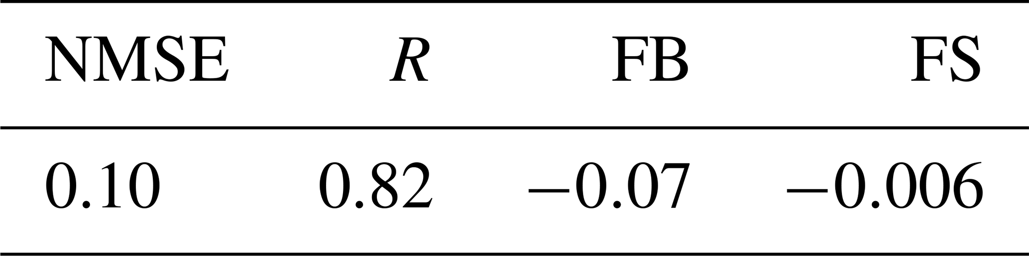
Table A3 exhibits Hanna's statistical indices, which are commonly used to calibrate air pollution dispersion models. Such indices are defined as

\begin{matrix} (16) & normalized mean square error (NMSE) = \frac{\overline{{(C_{o} - C_{p})}^{2}}}{\overline{C_{o} C_{p}}}, \\ (17) & correlation coefficient (R) = \frac{(C_{o} - \overline{C_{o}}) (C_{p} - \overline{C_{p}})}{σ_{o} σ_{p}}, \\ (18) & fractional bias (FB) = \frac{(\overline{C_{o}} - \overline{C_{p}})}{0.5 (\overline{C_{o}} + \overline{C_{p}})}, \\ (19) & fractional standard deviations (FS) = \frac{σ_{o} - σ_{p}}{0.5 (σ_{o} σ_{p})}, \end{matrix}

where C_p is the predicted concentration, C_o is the observed concentration, σ_p is the predicted standard deviation, σ_o is the observed standard deviation, and the overbar represents an averaged value.

The observed and predicted scatter diagram of concentrations in Fig. A1 demonstrates that the simulated concentration reproduces fairly well the measured concentration data. Furthermore, the statistical analysis of the results (Table A3) shows good agreement between the results of the proposed approach with the experimental ones. The indices are found within an acceptable interval, with NMSE (normalized mean square error), FB (fractional bias) and FS (fractional standard deviation) close to zero and R (correlation coefficient) near to one. These statistical indices show that the empirical eddy diffusivities obtained at a Brazilian coastal site can be used to simulate contaminant dispersion in other coastal areas. Thus, the present development based on an analysis of high-resolution turbulence data from an elevated micrometeorological tower provides suitable eddy diffusivities that describe the turbulent transport patterns in a CIBL.

3 Conclusions

The Eulerian operational air dispersion models that simulate contaminant observed concentration data need to incorporate into their formulation the characteristics of the PBL turbulent diffusion process. To accomplish this parameterization they use turbulent transport terms known as eddy diffusivities. These turbulent parameters represent approximate quantities which intend to reproduce the complex natural dispersive effects. In this study, algebraic expressions for quasi-experimental convective eddy diffusivities for a coastal site are derived. The derivation employed the Taylor statistical diffusion theory and sonic anemometer observations with high vertical resolution in a CIBL.

The complexity of the subject does not allow a direct confrontation between experiment and model. However, utilizing the APUGRID Eulerian dispersion model and a concentration data set of dispersion experiments performed in a CIBL, the derived eddy diffusivities have been tested and validated. The comparison results show that there is fairly good agreement between simulated and measured concentrations. As a consequence, the results provided in this investigation are encouraging. Thus, the new eddy diffusivities for a coastal site may be suitable for applications in regulatory air pollution modeling.

Appendix A

https://www.ann-geophys.net/38/603/2020/angeo-38-603-2020-f01

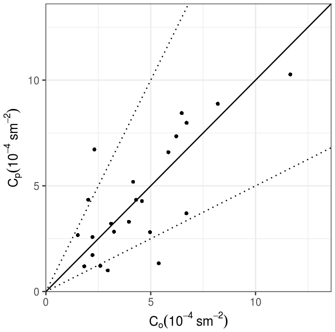
Figure A1Scatter diagram between Copenhagen observed (C_o∕Q) and predicted (C_p∕Q) ground-level crosswind-integrated concentrations normalized by the emission rate.

Download

Table A1Meteorological conditions during the Copenhagen dispersion experiments.

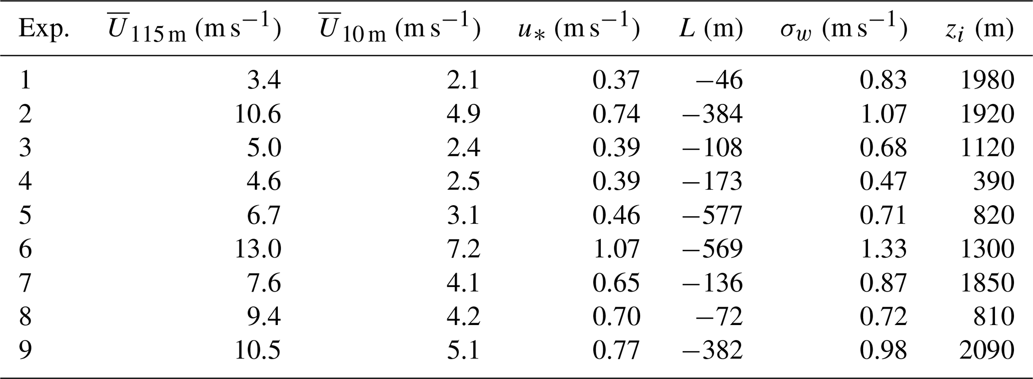
Download Print Version | Download XLSX

Table A2Observed C_o and predicted C_p crosswind-integrated concentrations normalized by the emission rate (Q) for Copenhagen experiments.

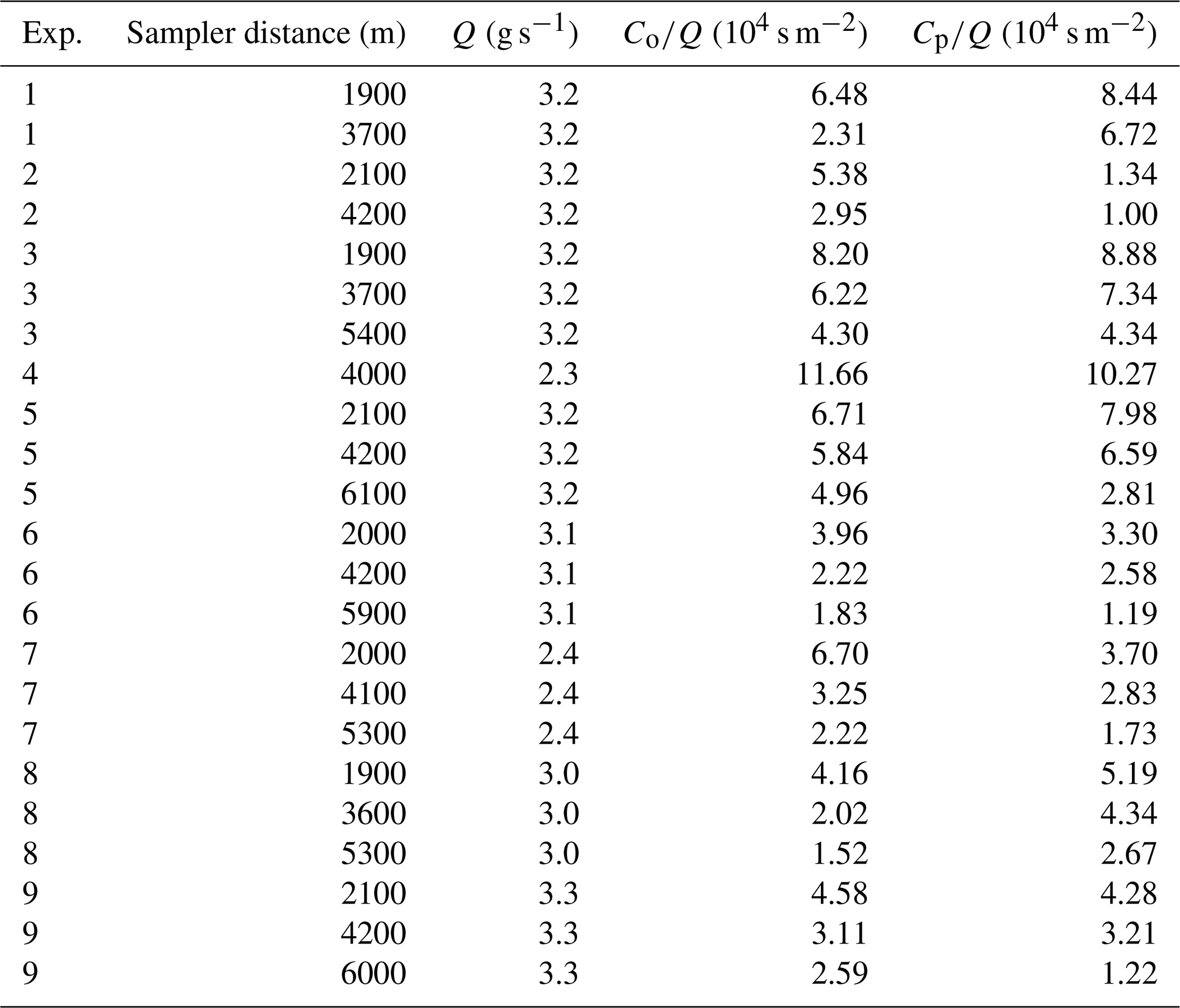
Download Print Version | Download XLSX

Table A3Statistical evaluation of the APUGRID model employing the quasi-experimental eddy diffusivities.

Download Print Version | Download XLSX

Data availability

The data used in this study are available by contacting the corresponding author (Gervásio Annes Degrazia, email: gervasiodegrazia@gmail.com).

Author contributions

SM, MS, LGNM, GAD, UR, DRR, FSP, and OCA performed the measurements and/or contributed to the data analysis. All the authors contributed to the discussion and interpretation of the results and writing the paper.

Competing interests

The authors declare that they have no conflict of interest.

Special issue statement

This article is part of the special issue “7th Brazilian meeting on space geophysics and aeronomy”. It is a result of the Brazilian meeting on Space Geophysics and Aeronomy, Santa Maria/RS, Brazil, 5–9 November 2018.

Financial support

This study has been developed within the context of a research and development project regulated by the Brazilian National Agency for Electric Energy and sponsored by the companies Linhares Geração S.A. and Termelétrica Viana S.A. The study also has been partially supported by Brazilian funding agencies CNPq, CAPES and FAPERGS.

Review statement

This paper was edited by Petr Pisoft and reviewed by three anonymous referees.

References

Batchelor, G. K.: Diffusion in a field of homogeneous turbulence. I. Eulerian analysis, Aust. J. Chem., 2, 437–450, https://doi.org/10.1071/CH9490437, 1949. a

Berkowicz, R., Olesen, H., and Torp, U.: The Danish Gaussian air pollution model (OML): Description, test and sensitivity analysis in view of regulatory applications, in: Air Pollution Modeling and Its Application V, 453–481, Springer, Boston, USA, 1986. a

Degrazia, G. and Anfossi, D.: Estimation of the Kolmogorov constant C₀ from classical statistical diffusion theory, Atmos. Environ., 32, 3611–3614, https://doi.org/10.1016/S1352-2310(98)00038-7, 1998. a

Degrazia, G., Anfossi, D., Carvalho, J., Mangia, C., Tirabassi, T., and Velho, H. C.: Turbulence parameterisation for PBL dispersion models in all stability conditions, Atmos. Environ., 34, 3575–3583, https://doi.org/10.1016/S1352-2310(00)00116-3, 2000. a

Degrazia, G. A., Moreira, D. M., and Vilhena, M. T.: Derivation of an eddy diffusivity depending on source distance for vertically inhomogeneous turbulence in a convective boundary layer, J. Appl. Meteorol., 40, 1233–1240, https://doi.org/10.1175/1520-0450(2001)040<1233:DOAEDD>2.0.CO;2, 2001. a

Durand, P., Druilhet, A., and Briere, S.: A sea-land transition observed during the COAST experiment, J. Atmos. Sci., 46, 96–116, https://doi.org/10.1175/1520-0469(1989)046<0096:ASLTOD>2.0.CO;2, 1989. a

Garratt, J. R.: The Atmospheric Boundary Layer, Univ. Press, New York, USA, 1992. a

Gryning, S.-E. and Lyck, E.: Atmospheric dispersion from elevated sources in an urban area: comparison between tracer experiments and model calculations, J. Clim. Appl. Meteorol., 23, 651–660, 1984. a

Hanna, S. R.: Lagrangian and Eulerian time-scale relations in the daytime boundary layer, J. Appl. Meteorol., 20, 242–249, 1981. a

Hanna, S. R., Briggs, G. A., Hosker Jr., R. P.: Handbook on atmospheric diffusion, National Oceanic and Atmospheric Administration, Oak Ridge, TN (USA), Atmospheric Turbulence and Diffusion Lab., 1982. a

Hara, T., Ohya, Y., Uchida, T., and Ohba, R.: Wind-tunnel and numerical simulations of the coastal thermal internal boundary layer, Bound.-Lay. Meteorol., 130, 365–381, https://doi.org/10.1007/s10546-008-9343-5, 2009. a

Hinze, J.: Turbulence, Vol. 218, McGraw-Hill, New York, 1975. a

Kaimal, J. C., Wyngaard, J., Izumi, Y., and Coté, O.: Spectral characteristics of surface-layer turbulence, Q. J. Roy. Meteor. Soc., 98, 563–589, https://doi.org/10.1002/qj.49709841707, 1972. a

Leelőssy, Á., Molnár, F., Izsák, F., Havasi, Á., Lagzi, I., and Mészáros, R.: Dispersion modeling of air pollutants in the atmosphere: a review, Open Geosci., 6, 257–278, 2014. a

Long, J. and Pepper, D.: An examination of some simple numerical schemes for calculating scalar advection, J. Appl. Meteorol., 20, 146–156, 1981. a

Mařcuk, G. I.: Metodi del calcolo numerico, Editori riuniti, Roma, 1984. a

Martins, L. G. N., Degrazia, G. A., Acevedo, O. C., Puhales, F. S., de Oliveira, P. E., Teichrieb, C. A., and da Silva, S. M.: Quasi-Experimental Determination of Turbulent Dispersion Parameters for Different Stability Conditions from a Tall Micrometeorological Tower, J. Appl. Meteorol. Clim., 57, 1729–1745, https://doi.org/10.1175/JAMC-D-17-0269.1, 2018. a, b, c, d, e

McRae, G. J., Goodin, W. R., and Seinfeld, J. H.: Numerical solution of the atmospheric diffusion equation for chemically reacting flows, J. Comput. Phys., 45, 1–42, https://doi.org/10.1016/0021-9991(82)90101-2, 1982. a, b

Ogawa, Y. and Ohara, T.: The turbulent structure of the internal boundary layer near the shore, Bound.-Lay. Meteorol., 31, 369–384, https://doi.org/10.1007/BF00120836, 1985. a

Panofsky, H. A. and Dutton, J.: Atmospheric Turbulence: Models and Methods for Engineering Applications, John Wiley & Sons, New York, 1984. a

Pasquill, F. and Smith, F.: Atmospheric diffusion, 3rd Edn., John Wiley and Sons, New York, USA, 1983. a

Rizza, U., Gioia, G., Mangia, C., and Marra, G. P.: Development of a grid-dispersion model in a large-eddy-simulation generated planetary boundary layer, Il Nuovo Cimento, 26, 297–309, 2003. a, b

Rizza, U., Gioia, G., Lacorata, G., Mangia, C., and Marra, G. P.: Atmospheric Dispersion with a Large-Eddy Simulation: Eulerian and Lagrangian Perspectives, in: Air Pollution and turbulence modelling and aplications, edited by: Moreira, D. and Vilhena, M., 237–268, CRC Press, Boca Raton, USA, 2010. a, b

Shao, Y., Hacker, J. M., and Schwerdtfeger, P.: The structure of turbulence in a coastal atmospheric boundary layer, Q. J. Roy. Meteor. Soc., 117, 1299–1324, https://doi.org/10.1002/qj.49711750209, 1991. a

Smedman, A.-S. and Hoegstroem, U.: Turbulent characteristics of a shallow convective internal boundary layer, Bound.-Lay. Meteorol., 25, 271–287, 1983. a

Tirabassi, T.: Mathematical Air Pollution Models: Eulerian Modelss, in: Air pollution and turbulence: modeling and applications, edited by: Moreira, D. and Vilhena, M., 131–156, CRC Press, Boca Raton, USA, 2009. a

Yanenko, N. N.: The method of fractional steps, Springer, New York, USA, 1971. a, b

Yordanov, D., Kolarova, M., Rizza, U., Mangia, C., Tirabassi, T., and Syrakov, D.: Evaluation of wind and turbulent parameterisations for short range air pollution modeling, Bulgarian Geophysical Journal, 32, 107–123, 2006. a, b

Zannetti, P.: Air pollution modeling: theories, computational methods and available software, Springer Science & Business Media, California, USA, 2013. a

Articles

Short summary

In this paper, quasi-empirical convective eddy diffusivity parameterizations for a coastal site are obtained. In the derivation we used Taylor's theory of statistical diffusion and sonic anemometer observations collected at 11 levels on a 140 m high tower in a convective planetary boundary layer. The test of the derived coefficients was solved by solving the equation of diffusion–advection by the fractional step/locally one-dimensional (LOD) methods.