2.1 The all-sky imager

The GWs detected in this study were observed using the ASI installed at the observatory in São João do Cariri. The ASI is an optical instrument that provides monochromatic maps of aurora and atmospheric airglow emissions at different wavelengths. It has been designed to keep track of the spatial and temporal variations of OH, OI 557.7 nm and OI630.0 nm airglow emissions (e.g. Paulino et al., 2010).

However, the present study only utilised the OH airglow images captured by the ASI at an altitude of 87 km. This instrument is comprised of a fish-eye (f/4) lens, a telecentric lens system, a field of view of 180^∘, a computer-controlled filter wheel with several slots for the observation of different emissions and a camera with a charge-coupled device (CCD) that is used as a photodetector to increase sensitivity. More technical and operational details about this particular imager at São João do Cariri can be found in previous works (Medeiros et al., 2007; Paulino et al., 2012).

2.2 SABER/TIMED satellite

The Sounding of the Atmosphere using Broadband Emission Radiometry (SABER) is one of the four instruments onboard the Thermosphere Ionosphere Mesosphere Energetics and Dynamics (TIMED) satellite. The vertical temperature measurements from 20 to 108 km were observed on 8 April 2005 over the São João do Cariri area (7.4^∘ S, 36.5^∘ W) from this instrument (SABER). Data from the Naval Research Laboratory Mass Spectrometer Incoherent Scatter (NRLMSISE00) atmospheric model (Picone et al., 2002) were utilised to supplement the measurements at unavailable heights, namely 0–19 and 109–400 km. These measurements were used to provide vertical profiles of kinetic temperature, pressure, geopotential height, and volume mixing ratios for the trace species (Mertens et al., 2001).

2.3 The SKiYMET meteor radar

The All-Sky Interferometric Meteor Radar (SKiYMET) system located at São João do Cariri (7.4^∘ S, 36.5^∘ W ) provided measurements of the horizontal wind speed and direction in the MLT (81–99 km). The radar is composed of Yagi antennas: five receiving antennas and one transmitting antenna that operate at 35.24 MHz with a maximum power of 12 kW. This instrument detects the trail left behind by vaporised meteors, determines the angle-of-arrival using the phase difference between the receiving antennas, and then measures the radial velocity using the derivation of the speed and direction of the atmospheric winds carrying the meteor trail at a specified altitude. The phase delay between the transmitted and received signal is used to determine the position of the trail. Further details about this radar are presented in previous works (e.g. Hocking et al., 2001; Egito et al., 2018; Paulino et al., 2015).

3.1 Determination of GW parameters

To obtain the characteristics of the detected GWs, a two-dimensional fast Fourier transform (FFT) was used in specified batches of OH airglow images. The preprocessing of the airglow images can be summarised using the following procedures:

• rotation of the image to fit the top of the image with the northern geographic region;

• removal of low-frequency waves by applying the Butterworth high-pass filter;

• contrast enhancement and unwarping of the airglow images for FFT analysis.

Figure 1a shows one of the raw OH images obtained from the São João do Cariri ASI at the Observatório de Luminescência Atmosférica de Paraiba (OLAP). This image is a typical example of the GWs observed during this night (8 April 2005). The ripples enclosed in the red box in Fig. 1a represent the GW structure. This particular GW was captured by the ASI at ∼ 23:58 UT on 8 April 2005. However, the image was contaminated by stars (bright circles), the Milky Way (white streak running from the bottom northwest in a southeasterly direction), tree branches/leaves (eastern edge of the image) and the tops of buildings (shown by the red arrow). Figure 1b portrays a clearer image after image processing; Fig. 1c represents the unwarped version of the previous image; Fig. 1d shows the spectrum of the encapsulated GW. The bright red circle that depicts the amplitude of the GW and its positioning also provides the propagation direction of the wave. Table 1 presents a summary of all of the GWs observed during this night. Additional information about the cross-spectrum analysis used in the present study to obtain the characteristics of these waves can be found in Wrasse et al. (2006).

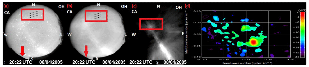
Figure 1Illustration of the image processing. (a) Raw OH image collected from the ASI in São João do Cariri on 8 April 2005. For more details on the propagation of ripples, see the video clip in the Supplement. (b) The filtered image. (c) The unwarped and rotated image of the GW event inside the red box shown in the previous images for FFT analysis (d) The cross spectrum applied to the GW enclosed in the red box in (c).

Download

Table 1The observed properties of the five GWs.

Download Print Version | Download XLSX

3.2 The atmospheric profile

The SABER instrument provided temperature measurements from 23:46 to 23:51 UT on 8 April and from 08:35 to 08:40 UT on 9 April for altitudes between 20 and 108 km. Linear interpolation was then carried out between 23:51 (8 April) and 08:35 UT (9 April) for the same altitude range. In addition, numerical values for temperature were obtained from the NRLMSISE-00 model for time (12:00 to 22:00) on 8 April 2005 and for missing heights (0–19 and 109–400 km) to supplement the SABER measurements. Finally, a 13-profile temperature dataset with a temporal resolution of 2 h was constructed for the whole period. However, some discrepancies were observed where points intersected; hence, the data were smoothened so that the model could seamlessly match the measurements at these junctions. This methodology was discussed by Paulino et al. (2012).

The SKiYMET radar provided the zonal and meridional wind measurements from 81 to 99 km every 3 km from 00:00 to 23:00 on 8 and 9 April 2005 at a temporal resolution of 1 h. Similarly, numerical interpolation was used to provide the spatial resolution of the wind at a 2 h temporal resolution, as for the temperature profile, with supporting data from the Horizontal Wind Model (HWM) (Drob et al., 2008) from 0 to 80 km, and above 100 km.

From the temperature and wind measurements, other atmospheric parameters representing the atmospheric state of the study period were obtained. The pressure $P\left(z\right)=P_{\mathrm{0}}{\exp }^{\left(-{\int }_{\mathrm{0}}^z\frac{g}{RT}\mathrm{d}z{}^{\prime }\right)}$ was obtained using a combination of the ideal gas law (P=RρT) and the hydrostatic balance equation ($\frac{\mathrm{d}P}{\mathrm{d}z}=-gp$, where ρ is the density obtained from the MSIS model); the molecular weight was estimated from $X_{\mathrm{MW}}=\frac{\mathrm{1}}{\mathrm{2}}\left(X_{\mathrm{MW}\mathrm{0}}-X_{\mathrm{MW}\mathrm{1}}\right)\left[\mathrm{1}-\tanh \frac{s-a}{{\mathrm{\Delta }}_a}\right]+X_{\mathrm{MW}\mathrm{1}}$, where X_MW0, X_MW1, Δ_a and a are constants given by 28.90, 16.0, 4.20, and 14.90 respectively, while s=ln ρ (Vadas et al., 2009). Additional details about the reverse ray-tracing parameters can be found in Vadas (2007) and Vadas et al. (2009). Briefly, T is the temperature, g is the acceleration due to gravity, $R=\frac{\mathrm{8314.5}}{X_{\mathrm{MW}}}$ is the gas constant, z is the altitude, and P₀ is the pressure when z=0 .

The scale height $H=-\mathit{\rho }/\mathrm{d}\mathit{\rho }/\mathrm{d}z$ is obtained from the ratio of the density to the derivative with respect to the altitude; the potential temperature is $\mathit{\theta }=T{\left(P_{\mathrm{0}}/P\right)}^{R/C_{\mathrm{p}}}$, where C_p is the specific heat capacity at constant pressure; the Brunt–Väisälä frequency is $N=\sqrt{\left(\frac{g}{\mathrm{\Theta }}\frac{\mathrm{d}\mathrm{\Theta }}{\mathrm{d}z}\right)}$. See Vadas (2007) for further details.

3.3 The reverse ray-tracing technique

Every GW is influenced by the atmospheric winds with a velocity $\mathit{V}=\left({\text{V}}_i,{\text{V}}_j,{\text{V}}_k\right)$ according to Eqs. (1) and (2). Equation (1) describes the ray path, and the refraction of the wave vector along the ray path is explained by Eq. (2). The tracing model employed in the study is based on Lighthill (1978).

and

where both i and $j=\mathrm{1},\mathrm{2},\mathrm{3}$, and the repeated indices imply a summation; V_i represents the zonal, meridional, and vertical wind components. The spatial position of the wave is represented by x, k is the wave vector, ω_Ir is the real part of the intrinsic frequency obtained using the dispersion relation in Eq. (3) of Pramitha et al. (2015) and c_g is the group velocity.

Numerical integration of the six ordinary differential equations, Eqs. (1)–(2), was performed using a fourth-order Runge–Kutta scheme (Press, 2007). All of the observed and intrinsic properties of the GWs and the parameters representing the atmospheric condition were fed into the reverse ray-tracing (RRT) model. Four stopping conditions that were imposed constantly checked the propagation of the GWs into the background winds. When any of the conditions were violated, the ray-tracing integration was terminated. The main stopping criteria are as follows: (i) if the group velocity of the GW is close to the speed of sound (c_g≥0.9c_s); (ii) if the real part of the intrinsic frequency tends to zero (ω_Ir→0); (iii) if the vertical wavelength is greater than the viscosity length or the dissipation of the GWs; and (iv) if the momentum flow of the GW $u_{\mathrm{GW}}{w}_{\mathrm{GW}}\left(z,t\right)\ge {\mathrm{10}}^{-\mathrm{5}}{u}_{\mathrm{GW}}{w}_{\mathrm{GW}}$ at the height of OH airglow (87 km). Extensive details of the reverse ray-tracing algorithm employed in this study have been published in Paulino et al. (2012) and Pramitha et al. (2015).

4.1 Spectral analysis result

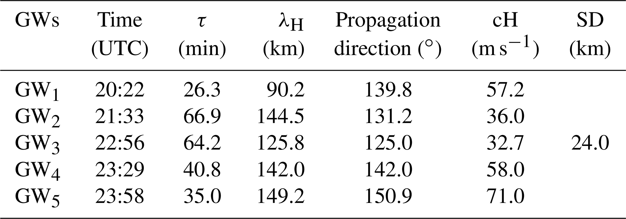
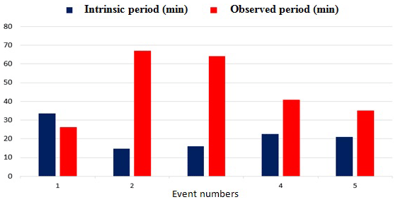
The spectral results in Table 1 show that the horizontal wavelengths (λ_H) have a standard deviation of 24 km and a mean value of 130 km with large variability among the detected waves, while the propagating period (τ) of the waves ranged from 26 to 67 min. These results agree with the reports of Medeiros et al. (2007) for waves detected at this observatory. Thus, it can be confidently concluded that the observed wavelengths are representative of the GWs at this observatory.

Figure 2 shows the travelling direction of the five GWs. From the polar chart, it is seen that all the waves are propagating southeast with an approximate azimuth of ∼134^∘ from the north. This is in favourable agreement with the results obtained from previous studies for the same observatory (Essien et al., 2018). This anisotropicity will be discussed later in this study.

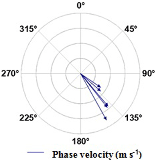
Figure 2Compass graph showing wave velocities and the direction of propagation – each circle denotes a velocity of 20 m s⁻¹.

Download

Figure 3 shows the impact of the atmospheric wind on the period of the waves. It reveals the difference between the intrinsic period of the waves, which lacks atmospheric impact, and the observed period, which is susceptible to the influence of the atmospheric winds. However, it can be seen that the winds accelerated almost all of the GWs. The fluctuation in the period can be attributed to the variability of the horizontal winds. When the GW is travelling antiparallel to the wind direction, the second term on the left side of this equation ${\mathit{\omega }}_{\mathrm{I}}={\mathit{\omega }}_o-k_{\mathrm{H}}{V}_{\mathrm{GW}}$ would become negative, consequently forcing the observed frequency to be smaller than the intrinsic frequency – this invariably results in an increase in the observed periods.

Figure 3Bar chart of the intrinsic and observed periods.

Download

One important finding from the spectral analysis is that there is a wide spectrum of GWs being generated. This strongly suggests that the source of these GWs must be large (Vadas and Fritts, 2009). In order to investigate the likely sources of these waves, the next section of this work presents and discusses the results from the ray tracing.

4.2 Reverse ray tracing (RRT)

These five waves have different spectral characteristics, and they were all also observed at different times. Using the reverse ray-tracing technique to back trace these GWs from the point of observation in the airglow layer to their generation source, we present the following results of the RRT analysis. During the backward tracing, we assumed that critical levels are not encountered, as explained in Sect. 3.3.

Panels (a) in Figs. 4–8 are the ray paths as a function of the altitude and time and describe the influence of various wind conditions on each GW event. The light cyan line indicates the trajectory of the GW under zero wind influence, whereas the black line shows the travel path of the wave under the influence of HWM wind. This provides a better understanding of the impact of atmospheric winds on the travel paths of GWs from the middle to the lower atmosphere. The cyan and black shaded circles represent the time of generation of these waves under zero and modelled wind scenarios respectively. The dashed cyan and solid black lines represent the trajectory of the waves under zero and modelled wind conditions respectively.

Panels (b) in Figs. 4–8, however, describe the wave path as a function of longitude–latitude, thereby providing a closer view of the exact generation point of these waves linearised over the map. The dark blue clouds represent the corresponding convective processes observed at the exact time that these GWs were detected. The black shaded triangle represents the precise location of the ASI at the OLAP.

Figure 4b shows a GW propagating southeastward. Under the modelled wind conditions, this wave was generated at 17:00 UT of the same day, whereas under zero wind influence, it was triggered at 16:30 UT. Thus, the atmospheric winds were favourable and accelerated the travel speed. Figure 4b zooms in on the actual source point of this wave. With a horizontal wavelength of 90 km and phase velocity of 57.2 m s⁻¹, the reverse ray-tracing result points to the source being in the northern region of the detection point (OLAP). Even though the HWM-14 winds and zero winds are not equal, the GWs propagated through a similar path under both wind conditions. Below 70 km, the GW propagates rapidly in the southeasterly direction, which could be due to the strong winds.

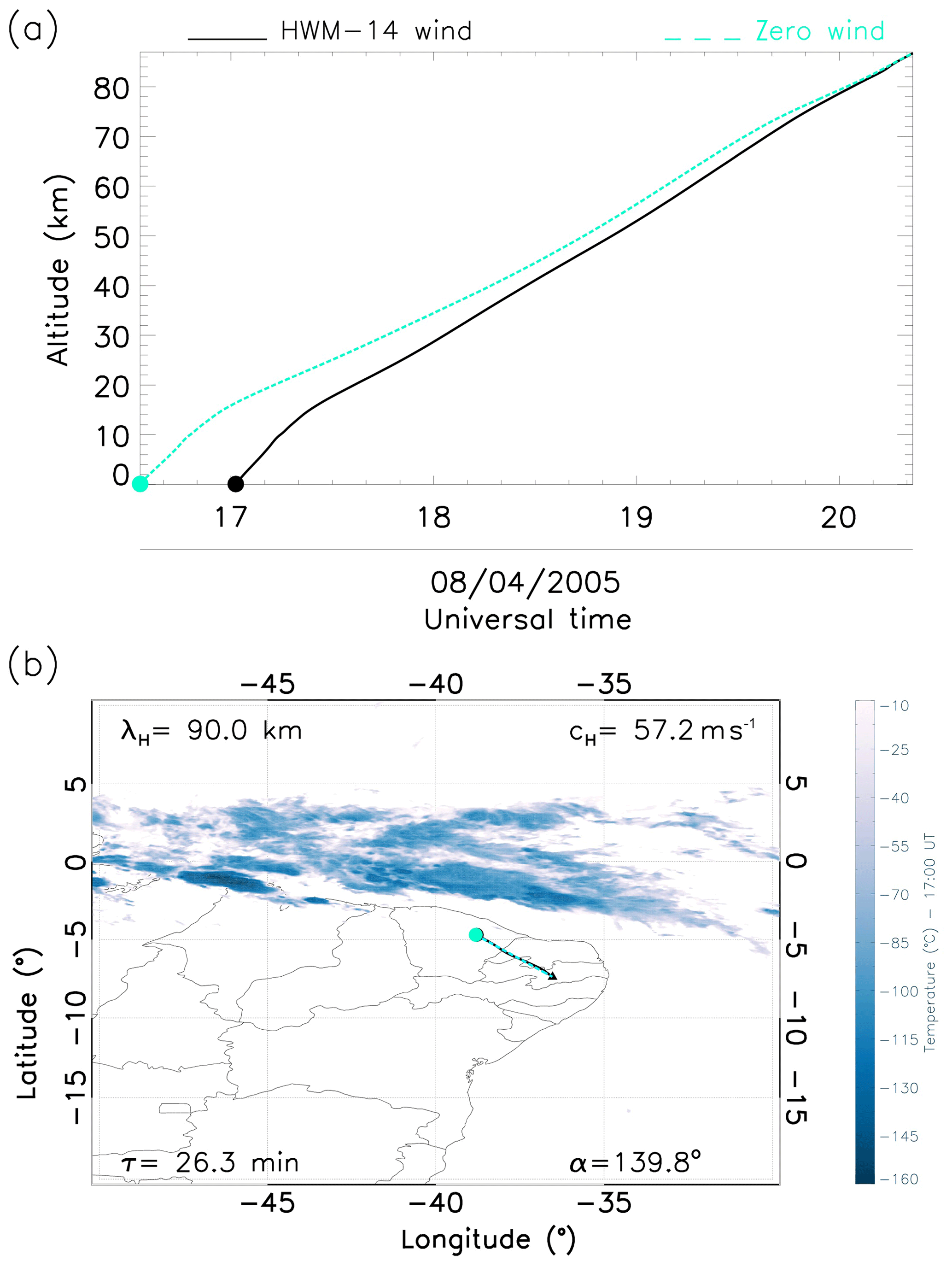
Figure 4Reverse ray-tracing results for GW₁. (a) Altitude as a function of time: dashed cyan and solid black lines show the ray paths for the zero winds and modelled winds respectively as well as the time cross section with zero wind and modelled winds. (b) Latitude–longitude cross section over convective cloud activities: black and cyan dots show the location of sources for zero winds and modelled winds respectively; the black triangle represents the exact location of the ASI, and the dark blue plumes represent convective activities in the region.

Download

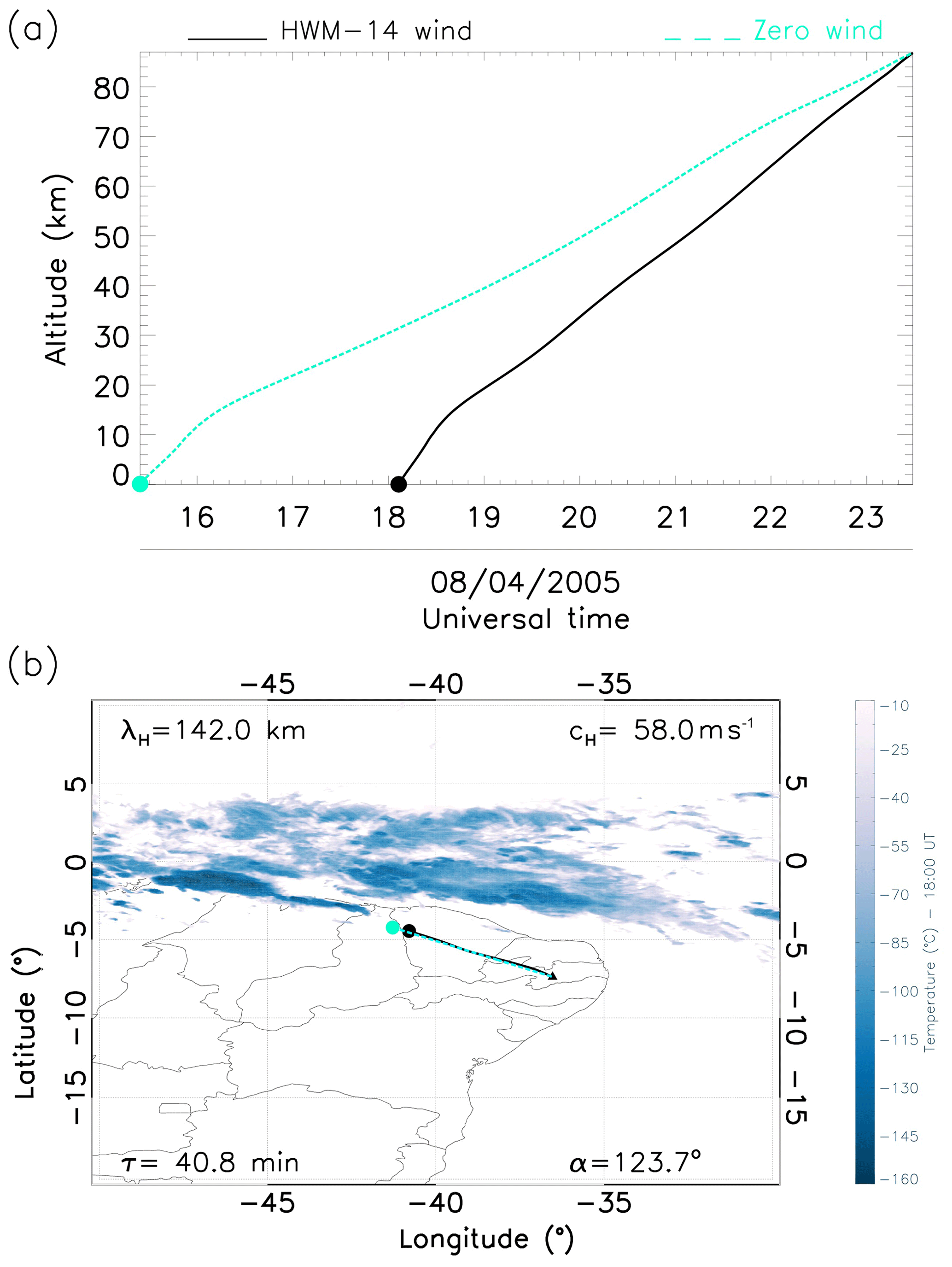
Similarly, the ray-tracing results show backward propagation of GW₂ that was detected at 21:33 UT (Fig. 5a). This shows a similar analysis to GW₁. However, GW₂ suffered greater wind acceleration ∼12 h, as did GW₃ ∼10 h. Moreover, just as in GW₁, both GW₄ and GW₅ were accelerated by the modelled winds by only ∼2 and 1 h respectively.

Figure 5Same as in Fig. 4 but for GW₂.

Download

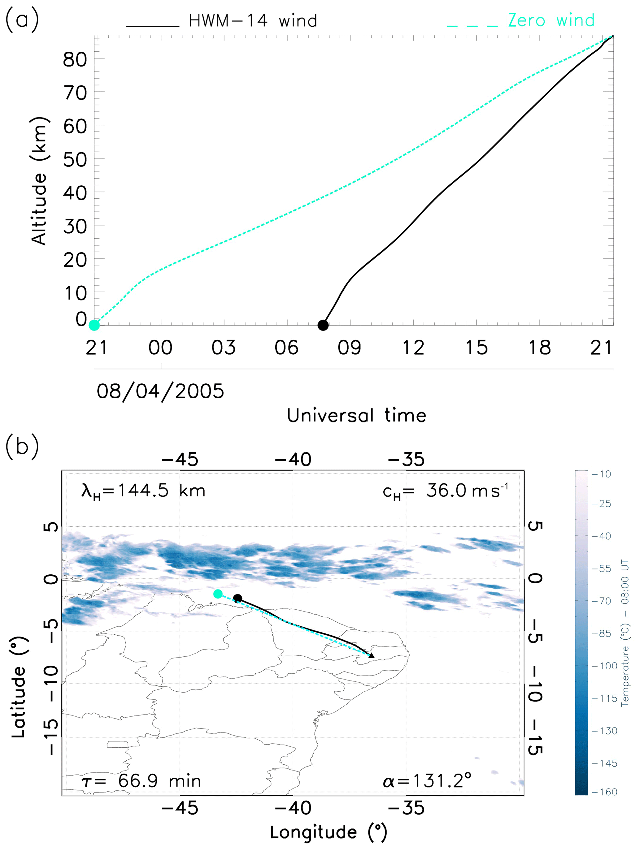
It was observed that GWs 2, 3, 4 and 5, which had mean horizontal wavelengths of 140 km, propagated more than ∼1300 km from their source region. All four of these GWs are believed to have originated from the same source due to the resemblance in their characteristics. In GW₁, in comparison to the others, the bottom side of the convective sources (dark blue clouds) appears to be farther from the point that we established (traced) as the GW's source (black and cyan dots). However, this particular wave is still linked to the convective processes as its source. According to Vadas and Fritts (2009), the actual convective area is usually larger than the cloudy areas.

Figure 6Same as Fig. 4 but for GW₃.

Download

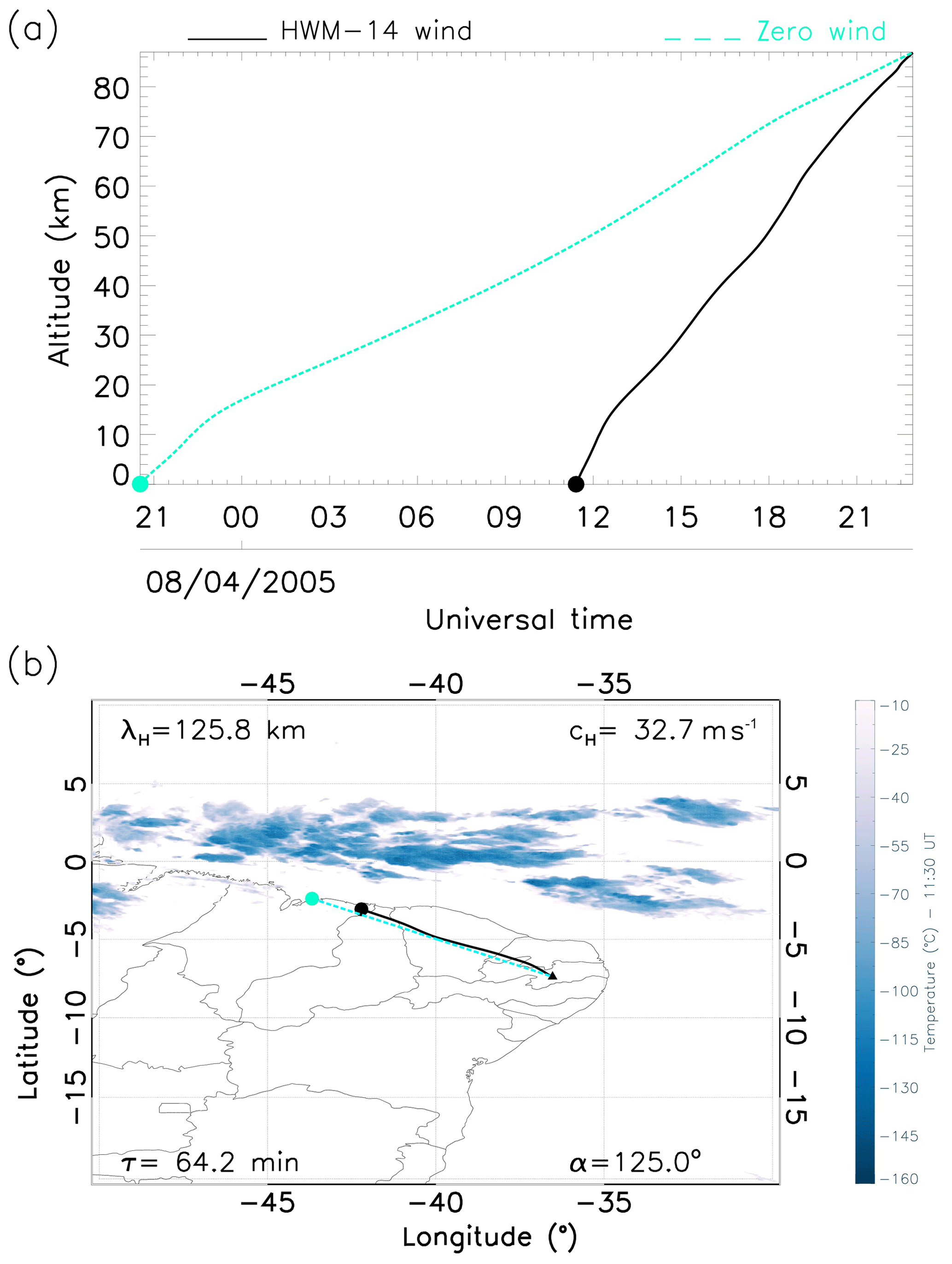
Figures 4b–8b showed the ray paths for the GWs, considering the normal and zero wind conditions. In the first panel of GW₃, the zero wind condition was applied, (cyan line) and the modelled wind condition (black line) was a horizontal wavelength of 90 km, a phase velocity of 57.2 m s⁻¹, a propagation angle of 139.8^∘, a 26.3 min period and a vertical wavelength of 90.2 km. In Fig. 6a, it can be noticed that GW₃ attained a height of 87 km for both wind conditions. A slight shift can be observed as there is a similarity between both conditions.

Figure 7Same as Fig. 4 but for GW₄.

Download

Figure 8Same as Fig. 5 but for GW₅.

Download

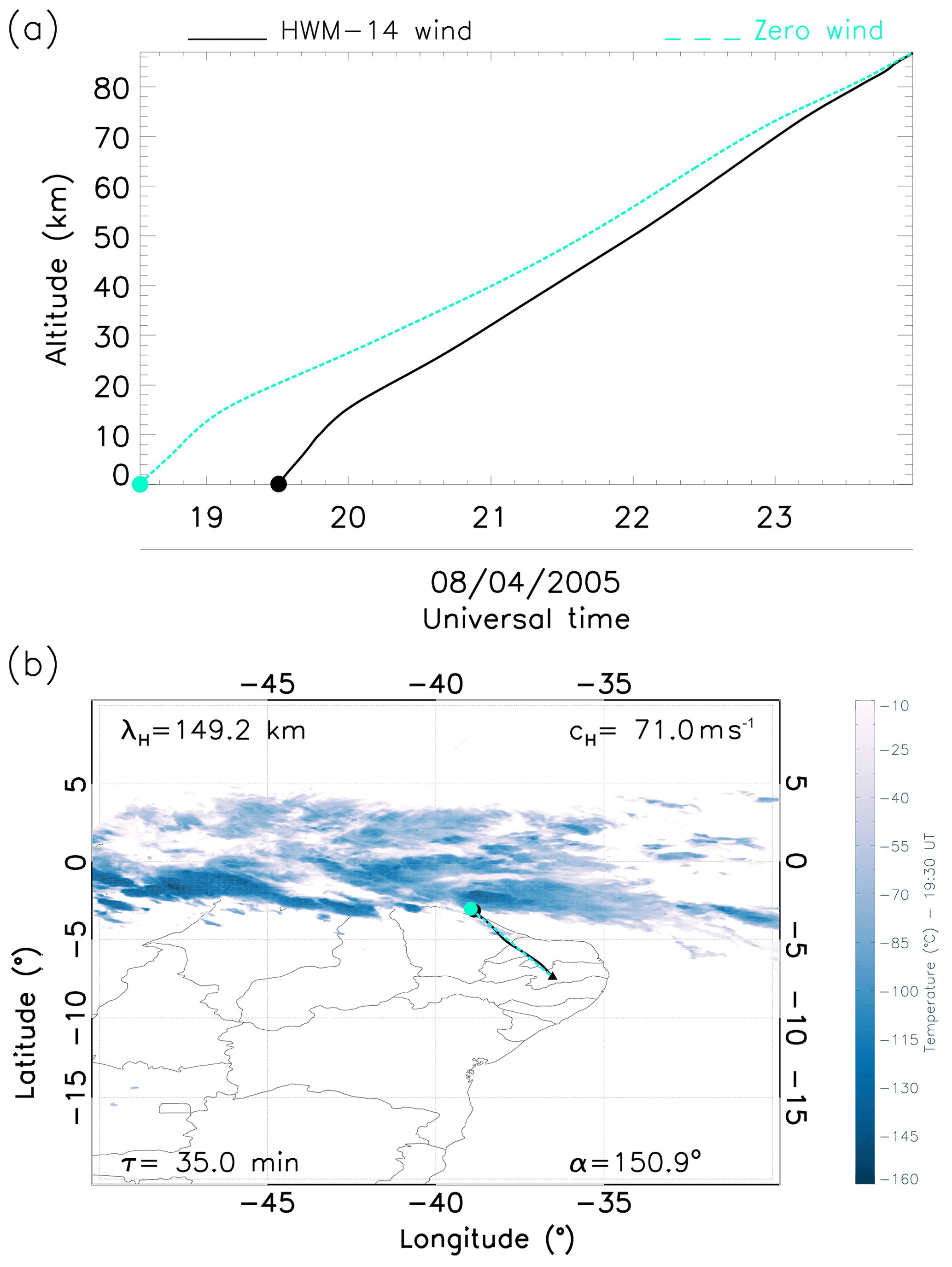
The five GWs were all traced back to convection activities occurring in the northern region of the OLAP observatory. These activities have been identified as possible generators of these waves. However, one question is evident: why do all of the waves propagate in a southeasterly direction when the Intertropical Convergence Zone (ITCZ) extends horizontally and covers the northern region of the observatory? These findings are in close agreement with previous results from different studies at this laboratory (e.g. Medeiros et al., 2003 and Essien et al., 2018). It is expected that the GWs should propagate in all directions in accordance with the location of the ITCZ. Thus, further investigation was carried out to explain this anisotropy. To better understand the physical mechanism that is producing the anisotropy, blocking diagrams have been used to investigate the role of the wind in the filtering process of these GWs.

Atmospheric winds are the default features of a real atmosphere. As these GWs propagate in the wind direction into the upper atmosphere, they become susceptible to the Doppler effect and critical level dissipation (Bretherton, 1966). The critical level marks the region where the horizontal wind component annuls the wave's horizontal phase speed (Medeiros et al., 2003). This region is very important, as it decides how and if a travelling wave would propagate further. To understand the anisotropy of these GWs, we apply the critical level theory of the atmospheric GW filtering (Fritts and Geller, 1976; Fritts, 1979). Based on the relation outlined by Gossard and Hooke (1975), the intrinsic frequency of the GW under the influence of both horizontal wind components can be described by Eq. (3) as follows:

where k is the magnitude of the horizontal wave vector, V represents the two horizontal wind components, and c is the horizontal phase speeds of the GWs. Equation (4) can also be re-expressed in terms of the zonal and meridional components. Further details can be found in the works of Medeiros et al. (2003), Campos et al. (2016) and Paulino et al. (2018). According to $\text{cH}=U\cos \mathrm{\varnothing }+V\sin \mathrm{\varnothing }$, where cH represents the phase speeds of these waves, U is the zonal wind component and V is the meridional wind component, we constructed blocking diagrams using the azimuthal angles (∅). With input winds from HWM, we aimed to understand the wind filtering effects on the GWs, to investigate why all of the waves had a preferential propagation direction, and also to detect regions where the phase speed of the GWs was less than or equal to the velocity of the winds. The results of the three-dimensional blocking diagrams are shown in Fig. 9.

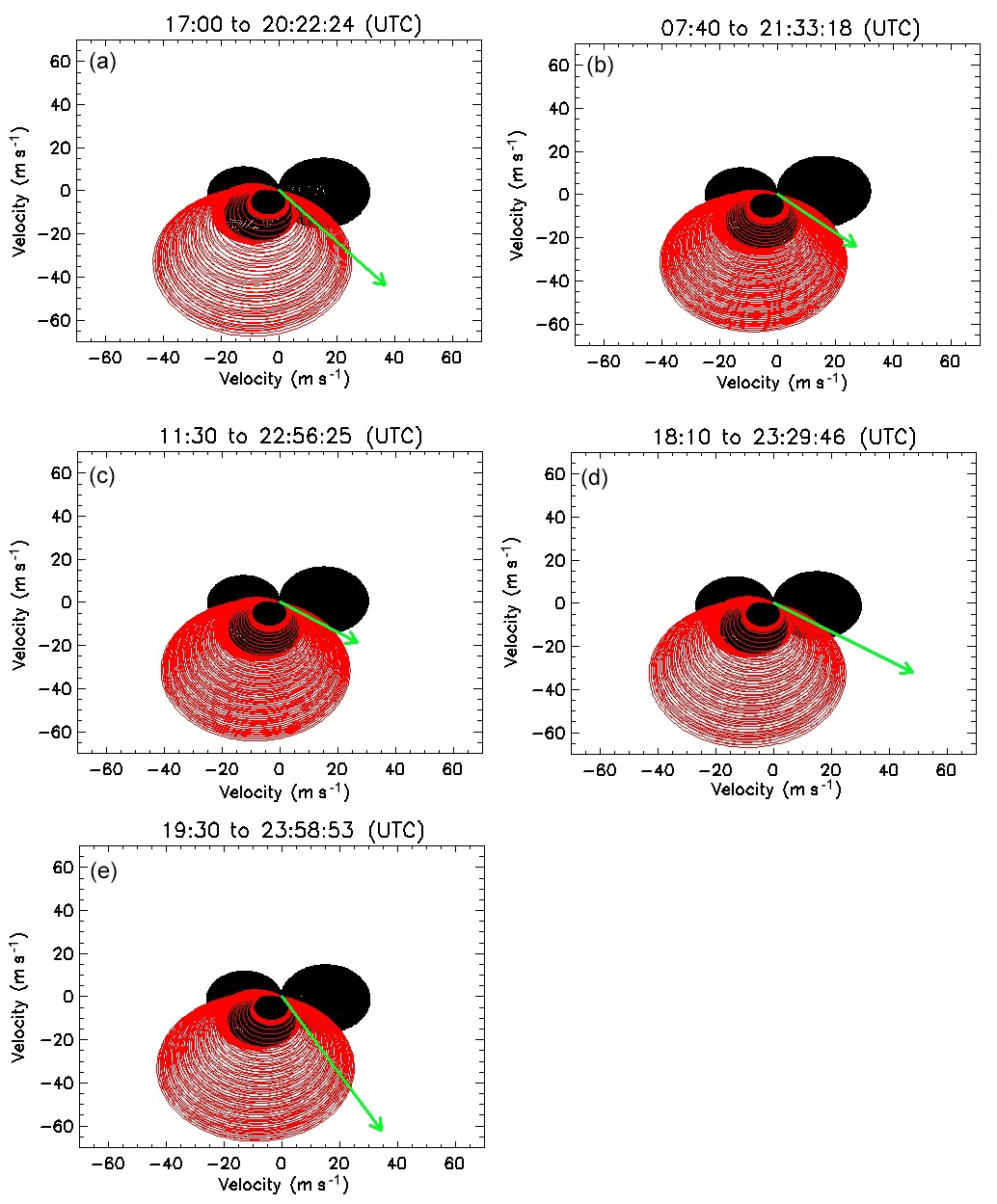
Figure 9(a) Two-dimensional blocking diagrams for the GW₁, (b) GW₂, (c) GW₃, (d) GW₄, and (e) GW₅ events observed in the OH layer (87 km). The green arrow depicts the magnitude and direction of the phase velocity of each GW. The red and black meshed regions represent the respective magnitude and the direction of the restricted area for the propagation of the wave to the (OH) layer.

Download

Constructing a polar chart as a function of the azimuthal angles and phase speeds using the wind data from HWM and the SKiYMET radar, we show where the phase speeds of these GWs equaled the wind speed of the background. The critical levels were projected into the blocking diagram for each horizontal wind speed and azimuth of the corresponding GWs. If the phase speed of the GW is trapped in the blocking lines, it represents that the wave is prohibited from propagating upwards.

Figure 9 allows the detection of regions where ω_I≤0 on the night of 8 April 2005 for the OH emission layer. Every circle in this diagram shows the critical level of the vertical propagation of these waves. The red and black meshed areas signify the measured and modelled wind components respectively, and the green arrow represents the magnitude and direction of the detected GW. The theory of the filtering process of GWs disallows wave propagation into the shaded region due to the effect of the critical levels (Paulino et al., 2018).

Similarly, we observed that the phase velocity of all of the GW events was indeed greater in magnitude than the blocking area. These GWs had strong speed and momentum, which was sufficient to escape and easily propagate through the critical levels. It is important to note the main contributions to the blocking area were due to the measured wind in the mesosphere and lower thermosphere, making this analysis strongly confident.

Thus, these detected waves avoided and escaped absorption in the forbidden regions by travelling at these interesting angles. Moreover, the anisotropy of these waves means that the source location of the wave must in the northwest, as the location of this wave source played a key role in this preferential travelling (Fritts et al., 2008; Campos et al., 2016). The sources of these waves were identified as the convective processes in the ITCZ zone.