Structural characterization of the equatorial F region plasma irregularities in the multifractal context

Joshi, Neelakshi; Rosa, Reinaldo R.; Savio, Siomel; Kherani, Esfhan Alam; de Meneses, Francisco Carlos; Stephany, Stephan; Muralikrishna, Polinaya

doi:https://doi.org/10.5194/angeo-38-445-2020

Articles | Volume 38, issue 2

https://doi.org/10.5194/angeo-38-445-2020

Special issue:

7th Brazilian meeting on space geophysics and aeronomy

https://doi.org/10.5194/angeo-38-445-2020

Articles | Volume 38, issue 2

Regular paper

03 Apr 2020

Regular paper |

| 03 Apr 2020

Structural characterization of the equatorial F region plasma irregularities in the multifractal context

Neelakshi Joshi, Reinaldo R. Rosa, Siomel Savio, Esfhan Alam Kherani, Francisco Carlos de Meneses, Stephan Stephany, and Polinaya Muralikrishna

Abstract

In the emerging ionosphere–space–weather paradigm, investigating the dynamical properties of ionospheric plasma irregularities using advanced computational nonlinear algorithms provide new insights into their turbulent-seeming nature, for instance, the evidence of energy distribution via a multiplicative cascade. In this study, we present a multifractal analysis of the equatorial F region in situ data obtained from two different experiments performed at Alcântara (2.4^∘ S, 44.4^∘ W), Brazil, to explore their scaling structures. The first experiment observed several medium- to large-scale plasma bubbles whereas the second experiment observed vertical uplift of the base of the F region. The multifractal detrended fluctuation analysis and the p-model fit are used to analyze the plasma density fluctuation time series. The result shows the presence of multifractality with degree of multifractality 0.53–0.93 and $0.3 \leq p \leq 0.4$ cascading probability for the first experiment. Other experimental data also exhibit multifractality with degree of multifractality 0.19–0.27 and $0.42 \leq p \leq 0.44$ cascading probability in ionospheric plasma irregularities. Our results confirm the nonhomogeneous nature of plasma irregularities and characterize the underlying nonhomogeneous multiplicative cascade hypothesis in the ionospheric medium. Differences in terms of scaling and complexity in the data belonging to different types of phenomena are also addressed.

Download & links

Article (PDF, 2164 KB)

How to cite

How to cite.

Dates

Received: 01 Sep 2019 – Discussion started: 25 Oct 2019 – Revised: 07 Jan 2020 – Accepted: 12 Feb 2020 – Published: 03 Apr 2020

1 Introduction

Present ionospheric research is transiting towards ionospheric space weather that goes beyond the ground- and space-based communication interruptions to influence decision-making communities on social, economical, and physical infrastructural policies. The enhancements in ionospheric plasma irregularities driven by space weather conditions demand an accurate characterization of the dynamical properties of the electron density and its complex nonlinear variation (Cander, 2019). With instruments operating over a substantial frequency domain, a study of plasma density irregularities provide insight into the underlying physical mechanism and its structural properties (Wernik et al., 2003; Muralikrishna et al., 2003). Energy dissipation is found to be an underlying process for the occurrence of electron density or electric field fluctuations in ionospheric plasma irregularities (Jahn and LaBelle, 1998; Kelley and Hysell, 1991).

Various rocket experiments and numerical simulations have been performed and contributed to our understanding of the generation and development of ionospheric irregularities. Costa and Kelley (1978) showed that the Rayleigh–Taylor instability that initiates in the bottomside equatorial F-region can nonlinearly develop very sharp gradients leading to the formation of steepened structures responsible for the power-law spectra observed by a rocket experiment in Natal, Brazil. Shock waves were observed by numerical simulation performed by Zargham and Seyler (1987) of the generalized Rayleigh–Taylor instability at the bottomside and topside F-region equatorial ionosphere, which was confirmed by rocket and satellite in situ data reported by Kelley et al. (1987). Hysell et al. (1994 a, b) proposed a model of plasma steepening, evolving from plasma advection that occurs on the vertical leading edges of plasma depletion wedges, to interpret shock waves detected in the equatorial ionosphere by rockets launched from Kwajalein Atoll. Jahn and LaBelle (1998) measured shock-like structures characterized by the density waveforms at the bottomside and topside F-region of the equatorial ionosphere in a rocket experiment in Alcântara, Brazil.

The spectral analysis, though widely used, falls short in characterizing nonstationary data as stationarity is assumed in the data, which is equivalent to presuming homogeneous turbulence; hence, a more robust method is necessary to analyze nonstationary data (Wernik et al., 2003). In addition, to develop a robust specification and a forecasting model, along with classical morphological, statistical, and spectral studies, a thorough understanding of nonlinearity in ionospheric irregularities is essential (Tanna and Pathak, 2014).

Recent advances in the computational algorithms based on fractal formalism, supplemented with mathematical modeling derived from probabilistic measures, have conclusively substantiated the occurrence of the energy cascading process in turbulent sites in the solar and interplanetary environment as well as in the laboratory using Kolmogorov's formalism as the basis (Grauer et al., 1994; Carbone et al., 1995; Abramenko et al., 2002; Macek, 2007; Wawrzaszek and Macek, 2010; Chian and Muñoz, 2011; Miranda et al., 2013; Wawrzaszek et al., 2019).

Various different approaches had been explored to understand nonlinear characteristics and intermittency in ionospheric irregularities, like structure function analysis (Dyrud et al., 2008; Spicher et al., 2015), fractal and multifractal analysis (Wernik et al., 2003; Alimov et al., 2008; Bolzan et al., 2013; Tanna and Pathak, 2014; Miriyala et al., 2015; Chandrasekhar et al., 2016; Fornari et al., 2016; Sivavaraprasad et al., 2018; Neelakshi et al., 2019), and multispectral optical imaging (Chian et al., 2018).

Structure function analysis performed on ionospheric high-latitude in situ data have revealed the intermittent nature of ionospheric irregularities owing to the large deviations from the Kolmogorov's K41 universal power-law index proposed for neutral fluid turbulence (Spicher et al., 2015).

In all the abovementioned studies, the main feature which gets highlighted is that the power spectra point to large deviations from the homogeneous turbulence described by the Kolmogorov spectrum ( $- 5 / 3$ ). Also, higher-order statistics like structure function analysis confirmed the deviation from the Kolmogorov scales, thus affirming the nonhomogeneity and intermittency in ionospheric irregularities. In the complex scenario of ionospheric turbulence, an important question that arises in the context of this paper is “is nonhomogeneity, which can be characterized by multifractal spectra, the cause for the large deviations from the $- 5 / 3$ ?” To answer this question, we propose using the multifractal detrended fluctuation analysis (MFDFA) on the equatorial F region plasma irregularities.

A detrended fluctuation analysis (DFA; Peng et al., 1994) has been a proven successful method to find a power law correlation and monofractal scaling in noisy, nonstationary data. The DFA is a robust method as it can handle discontinuous and length-wise short data. In case data are more complex and have intricate scaling, various scaling exponents characterize different parts of the data. To characterize such multiple scaling behavior in the data, Kantelhardt et al. (2002) generalized DFA to MFDFA, and have shown the equivalence to standard partition-function-based multifractal method for stationary data with compact support.

The MFDFA has wide applications in many branches of science, such as medicine (Makowiec, 2011), physics (de Freitas et al., 2016), engineering (Lu et al., 2016), finance (Grech, 2016), and social sciences (Kantelhardt, 2009; Telesca and Lovallo, 2011), to understand the complexity of a system through its scaling exponents that characterize multifractal dynamics of the system. The MFDFA has been applied to study ionospheric scintillation index time series (Tanna and Pathak, 2014; Miriyala et al., 2015) and ionospheric total electron content data (Chandrasekhar et al., 2016; Sivavaraprasad et al., 2018). For example, a wavelet transform was applied to study ionospheric irregularities (Wernik et al., 2003; Bolzan et al., 2013). These analyses identified multifractality and intermittency in nonlinear ionospheric irregularities.

In this work, we explore the low-latitude equatorial F region in situ data obtained from two different experiments and performed from the same rocket launching station. In the first experiment, done on 18 December 1995, the rocket traversed through various medium- to large-scale plasma irregularities during its descent, which were associated with the generalized Rayleigh–Taylor instability (Muralikrishna et al., 2003), whereas in the second experiment, done on 8 December 2012, the base of the F region was moving upward; i.e., pre-reversal enhancement (PRE) of vertical plasma drift was observed (Savio et al., 2016; Savio Odriozola et al., 2017).

In the equatorial ionosphere, the evening PRE is considered as an important seeding mechanism for the post-sunset F region irregularities, as quick and acute uplift of the electric field escalates the rate of growth of the generalized Rayleigh–Taylor instability (Li et al., 2007; Kelley et al., 2009; Abdu et al., 2018). Knowing the relation between these two phenomena, it will be interesting to know the differences in their scaling behavior and complexity. Investigating these plasma fluctuations may enable the study of the scaling properties of these plasma irregularities, and also knowing various characteristics along with the complexity of the data may provide important inputs to model empirical data. Hence, we apply the MFDFA method to the plasma density fluctuation data obtained from these two different in situ experiments. To corroborate our results, a multifractal spectrum obtained from the MFDFA is fitted with the p-model (Meneveau and Sreenivasan, 1987) based on the generalized two-scale Cantor set. Details on the experiments are given briefly in Sect. 2. Methods are described in Sect. 3. The results of the analyses are discussed in Sect. 4 followed by concluding remarks in Sect. 5.

2 In situ experiments

The equatorial launching station of Brazil is located at Alcântara (2.24^∘ S, 44.4^∘ W, dip latitude 5.5^∘ S). The SONDA III rocket was launched at 21:17 LT on 18 December 1995 under favorable conditions for formation of a plasma bubble. During the ∼11 min flight, the plane of rocket trajectory was almost orthogonal to the geomagnetic field lines and spanned ∼589 km distance horizontally with an apogee at altitude ∼557 km. A rocket-born electric field double probe (EFP) measured electric field fluctuations related to ionospheric plasma irregularities. In the upleg profile (ascent of the rocket), the F region base is clearly observed around 300 km, but without any large-scale depletion or bubble. On the other hand, several plasma bubbles of medium–large scale were observed in the downleg profile (descent of the rocket), around the base of F region and also topside of it, but without any sharp indication of the F region base from an altitude above 240 km. The rocket traversed through regions of different altitudes separated by a few hundred kilometers during upleg and downleg, so this might elucidate the large differences observed in ascent and descent of the rocket (Muralikrishna et al., 2003; Muralikrishna and Abdu, 2006; Muralikrishna and Vieira, 2007). A detailed explanation of in situ experiment and the analysis is found in Muralikrishna et al. (2003), Muralikrishna and Abdu (2006), and Muralikrishna and Vieira (2007).

Some of the key results from the aforementioned (Muralikrishna et al., 2003; Muralikrishna and Abdu, 2006; Muralikrishna and Vieira, 2007) analyses indicate (1) the initiation of a cascade process, owing to the generalized Rayleigh–Taylor instability mechanism near the base of F region that resulted in the development of plasma bubbles or large-scale irregularities, and (2) subsequently, when energy was advected to higher altitudes, smaller-scale irregularities were observed, owing to the cross-field instability mechanism.

From the same rocket launching station, Alcântara, a two-stage VS-30 Orion sounding rocket was launched at 19:00 LT, on 8 December 2012, under favorable conditions for strong spread F. During the ∼11 min flight, the rocket trajectory was in the north-northeast direction towards the magnetic equator, ranging ∼384 km horizontally with an apogee at ∼428 km. A conical Langmuir probe on board the rocket measured the electron density fluctuations associated with ionospheric plasma irregularities. In this experiment, the F region base was clearly observed in the downleg profile around 300 km, with some small-scale fluctuations in the F region. At the rocket launch time, the ground equipment, a digisonde, was operated from the equatorial station and reported fast uplift of the base of F layer, thus indicating the pre-reversal enhancement of the F region vertical drift (Savio et al., 2016; Savio Odriozola et al., 2017). Further explanation of the in situ experiment and data analysis is found in Savio et al. (2016); Savio Odriozola et al. (2017).

3 Methods

3.1 Multifractal detrended fluctuation analysis

Multifractal detrended fluctuation analysis (Kantelhardt et al., 2002) has been applied to investigate the multifractal properties of ionospheric irregularities in the following way.

To implement the MFDFA, a plasma density time series x_k of length N is considered. A first step is to compute the profile, Y(i), by calculating the cumulative sum by subtracting its mean.

\begin{matrix} (1) & Y (i) = \sum_{k = 1}^{i} [x_{k} - 〈 x 〉], i = 1, \dots, N \end{matrix}

divide the integrated profile into non-overlapping and equidistant N_s segments of s elements, referred to as scales. The length of the series may not be a multiple of all scales and a small part of the profile may be left out. To avoid it, repeat the same procedure over the profile but starting from the endpoint, in the reverse direction.

Now we have a total of 2N_s segments. These segments are then detrended using linear least squares. The variance is calculated over all segments:

\begin{matrix} (2) & \begin{aligned} F^{2} (s, v) = (\frac{1}{s} \sum_{i = 1}^{s} [Y [(v - 1) s + i] - y_{v} (i)]^{2}) \\ for each segment v, v = 1, 2, \dots, N_{s} \end{aligned} \end{matrix}

and

\begin{matrix} (3) & \begin{aligned} F^{2} (s, v) = (\frac{1}{s} \sum_{i = 1}^{s} [Y [N - (v - N_{s}) s + i] - y_{v} (i)]^{2}) \\ for each segment v, v = N_{s} + 1, \dots, 2 N_{s} . \end{aligned} \end{matrix}

y_v(i) is a polynomial fit obtained on a segment v. Now, averaging over all segments, the qth-order fluctuation function is computed.

\begin{matrix} (4) & \begin{aligned} F_{q} (s) = {(\frac{1}{2 N_{s}} \sum_{v = 1}^{2 N_{s}} [F^{2} (s, v)]^{q / 2})}^{1 / q} \\ for q \neq 0 \end{aligned} \end{matrix}

When q=0, logarithmic averaging should be used to calculate fluctuation function.

\begin{matrix} (5) & F_{0} (s) = \exp (\frac{1}{2 N_{s}} \sum_{v = 1}^{2 N_{s}} [\ln (F^{2} (s, v))]) \end{matrix}

Applying a linear fit to the fluctuation function profile on the log-log plot yields the generalized Hurst exponent, h(q), for each moment q as F_q(s)∝s^h(q). The computed generalized Hurst exponent h(q) can be related to the classical multifractal scaling (or mass) exponent as τ(q) by $τ (q) = q h (q) - 1$ . The multifractal spectrum is calculated using h(q) as follows:

\begin{matrix} (6) & α = h (q) + q h^{'} (q) where h^{'} (q) = \frac{d h}{d q}, \end{matrix}

\begin{matrix} (7) & f (α) = q (α - h (q)) + 1, \end{matrix}

where α represents the multifractal strength and f(α) represents a set of multifractal dimensions.

3.2 The p-model

The p-model is proposed by Meneveau and Sreenivasan (1987) to model the energy cascading process in the inertial range of fully developed turbulence for the dissipation field. The p-model starts with a coherent structure with an assumed specific energy flux per unit length which then undergoes a binary fragmentation at each cascading step, distributing the energy flux with probabilities p₁ and p₂ among the fragments l₁ and l₂. In this cascading process, n denotes the number of generations. In each generation, the segment size is given by $l_{1}^{m} l_{2}^{n - m}$ , where m denotes the number of left-side fragments and n−m represents right-side fragments in a segment (Halsey et al., 1986). An analytical formulation for the generalized two-scale Cantor set is given by

\begin{matrix} (8) & α = \frac{\ln (p_{1}) + (n / m - 1) \ln (p_{2})}{\ln (l_{1}) + (n / m - 1) \ln (l_{2})}, \end{matrix}

\begin{matrix} (9) & f (α) = \frac{(n / m - 1) \ln (n / m - 1) - (n / m) \ln (n / m)}{\ln (l_{1}) + (n / m - 1) \ln (l_{2})} . \end{matrix}

This is useful to determine the generalized multifractal dimensions which represent the multifractal spectrum (Halsey et al., 1986).

Based on the generalized two-scale Cantor set, the p-model consider equal fragment length (l₁=l₂) and unequal weights (p₁≠p₂ and $p_{1} + p_{2} \leq 1$ ). When $p_{1} + p_{2} \leq 1$ , loss in p parameter given by $d p = 1 - p_{1} - p_{2}$ , accounts for the direct energy dissipation in the energy cascading process in the inertial range. The proposed p-model claims to display all multifractal properties of one-dimensional section of the dissipation field for fully developed turbulence. The multifractality ceases to exist for p=0.5.

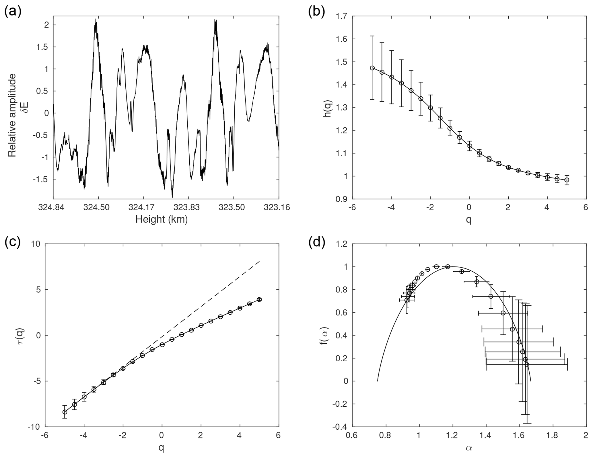
https://www.ann-geophys.net/38/445/2020/angeo-38-445-2020-f01

Figure 1Comprehensive MFDFA for the first experiment: panel (a) shows the time series at mean height 324.00 km and panel (b) shows the h(q) vs. q profile. Panel (c) shows τ(q) vs. q profile along with a dashed line which represents a linear relationship between τ(q) and q, and panel (d) shows the multifractal spectrum fitted with the p-model (continuous line).

Download

Table 1Multifractal analysis measures for the first experiment: the time series at mean heights are listed in the first column, the second column shows the degree of multifractality (Δα), and the third column gives the measure of asymmetry (A). Columns 4 to 6 list the p-model fit parameters, l₁, p₁, and dp respectively.

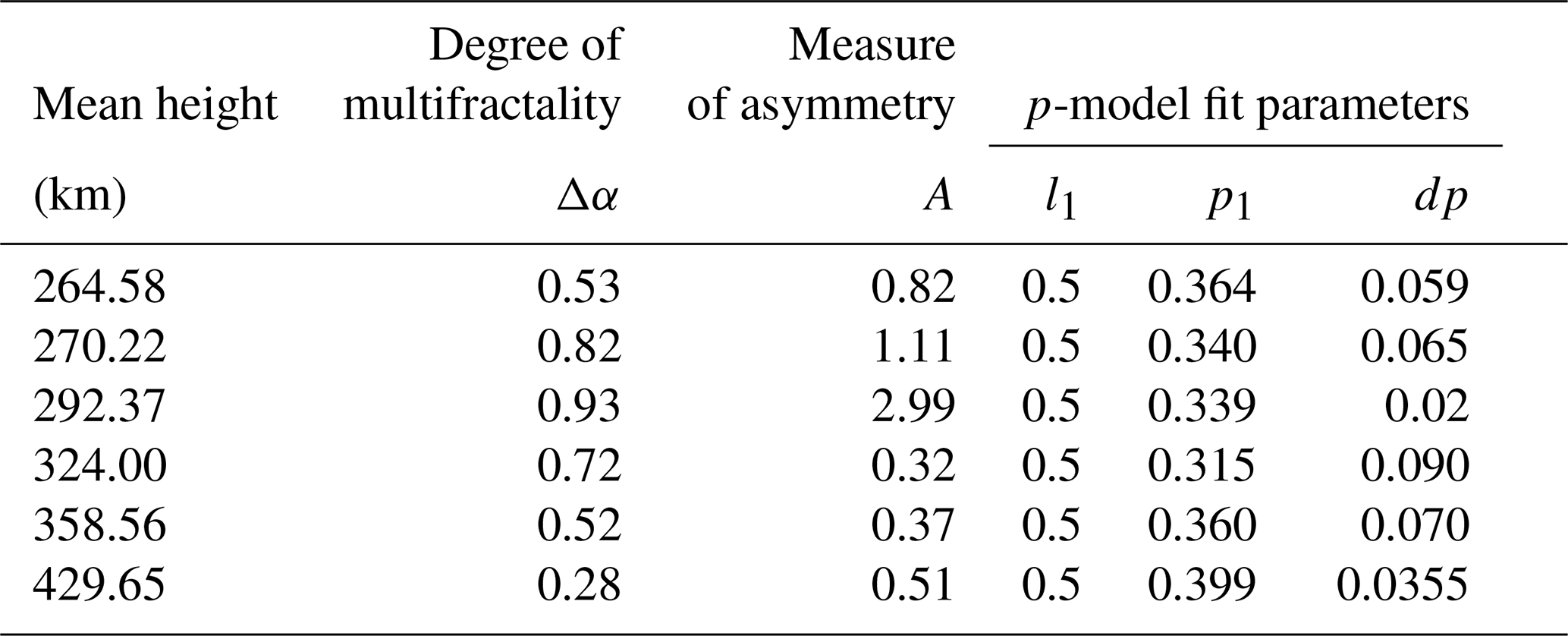
Download Print Version | Download XLSX

4 Results and interpretation

Six time series of in situ observations of electric field fluctuations from the F region are selected from the first experiment performed on 18 December 1995, corresponding to the mean heights of 264.58, 270.22, 292.37, 324.00, 358.56, and 429.65 km in the downleg. Similarly, from the second experiment performed on 12 December 2012, we selected three time series of electron density fluctuations from the F region, corresponding to the mean heights of 339.94, 348.99, and 400.24 km in the downleg. These time series are subjected to the multifractal analysis. Primarily, the profile is obtained by differencing the time series, i.e., $y = x (i + 1) - x (i)$ , using the criterion based on the power exponent obtained in the DFA method, prescribed by Ihlen (2012) in Table 2, for biomedical time series, to yield the best results from the MFDFA method. We found the criterion to hold for ionospheric in situ data under study. Scales up to 1∕10 of the length of the time series are considered. From the MFDFA, the generalized Hurst exponent h(q), classical multifractal scaling exponent τ(q) and multifractal spectrum α, and f(α) are obtained. We show a comprehensive analysis for only one time series from each of the two experiments (Figs. 1 and 2). For the remaining time series, we show only the multifractal spectrum along with its respective time series (Figs. 3 and 4), but we report the analysis of both experiments in Tables 1 and 2, respectively.

Table 2Multifractal analysis measures for the second experiment: For the time series at mean heights listed in the first column, the second column shows degree of multifractality (Δα), the third column gives measure of asymmetry (A). Columns 4 to 6 lists the p-model fit parameters, l₁, p₁, dp respectively.

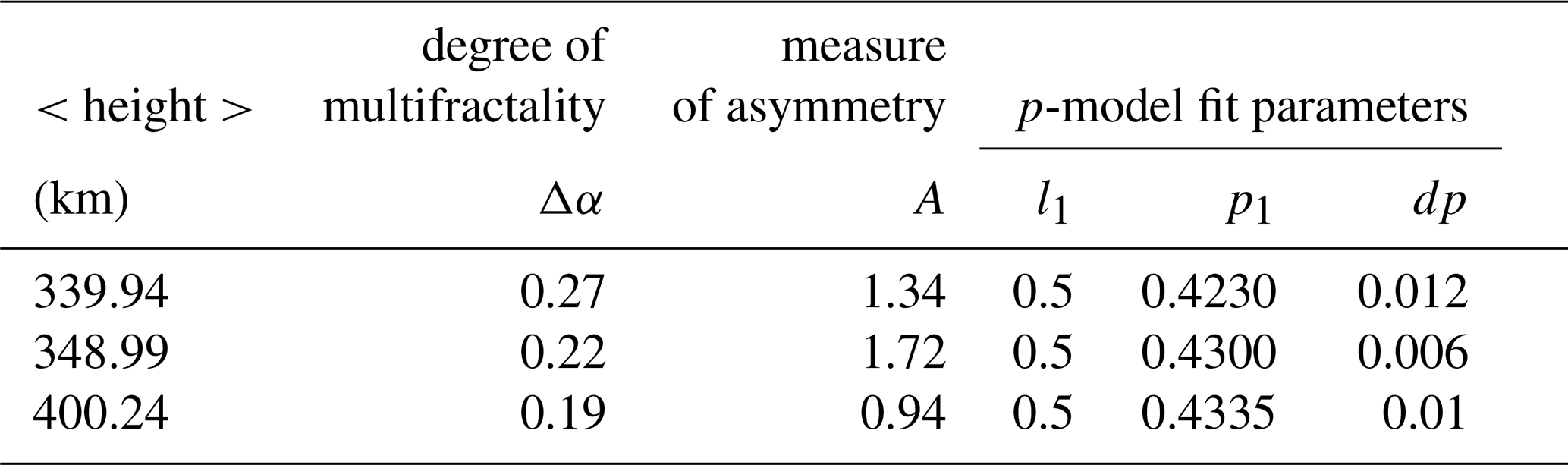
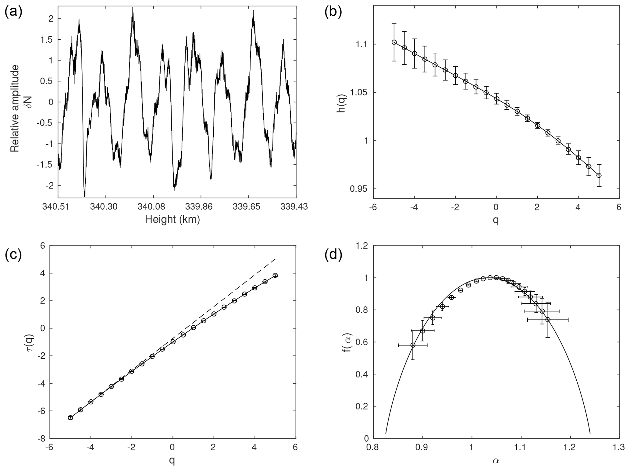
Download Print Version | Download XLSX

https://www.ann-geophys.net/38/445/2020/angeo-38-445-2020-f02

Figure 2Comprehensive MFDFA for the second experiment: panel (a) shows the time series at mean height 339.94 km and panel (b) shows the h(q) vs. q profile. Panel (c) shows the τ(q) vs. q profile along with a dashed line which represents a linear relationship between τ(q) and q, and panel (d) shows the multifractal spectrum fitted with the p-model (continuous line).

Download

In the MFDFA, fluctuation function Fq(s) is obtained by computing the qth-order local root mean square (RMS) for multiple segment size, i.e., for scales s. A segment may contain smaller to larger fluctuations. Rapid variation in fluctuations influence overall RMS for smaller-scale sizes, whereas slow variation in fluctuations influence overall RMS for larger-scale sizes. Negative q values characterize smaller fluctuations and positive q values characterize larger fluctuations in a segment. When q=0, it behaves neutrally. h(q) has dependence on q. To outline, for a multifractal time series h(q) monotonically decreases with q, and τ(q) shows nonlinear dependence on q. With q=0 as a center point, let us inspect how h(q) varies with respect to negative and positive values of q. If the time series is influenced by smaller fluctuations, then variation of h(q) for negative q will be faster, i.e., a steeper slope can be observed with respect to negative q and vice versa (Kantelhardt et al., 2002; Ihlen, 2012).

The multifractal spectrum illustrates how segments with small and large fluctuations deviate from the average fractal structure. The shape and width of the multifractal spectrum are also important measures to quantify the nature of multifractality present in the data. For f(α)=1, the corresponding value of α, known as α₀, divides the spectrum into left and right sides. A shape of the spectrum (the difference between the left and right sides of the spectrum) can be quantified by measure of asymmetry, A, given by

\begin{matrix} (10) & A = \frac{α_{0} - α_{min}}{α_{max} - α_{0}} . \end{matrix}

When A=1, the multifractal spectrum is symmetric in the sense that the time series is influenced by both larger as well as smaller fluctuations. When A>1, the spectrum is left-skewed, which implies that the time series is more influenced by the larger fluctuations. When A<1, the spectrum is right-skewed, which implies that the time series is more influenced by smaller fluctuations.

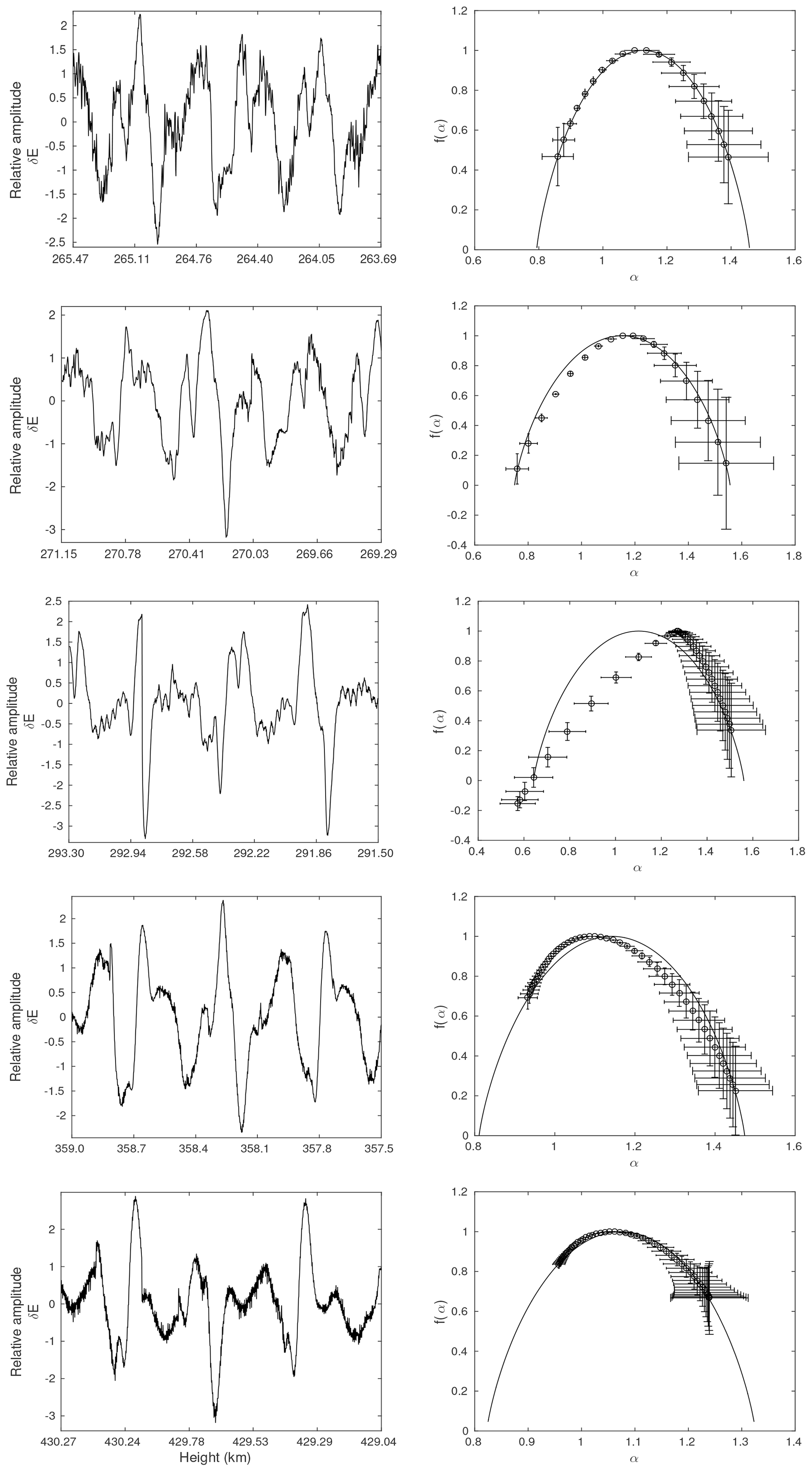
https://www.ann-geophys.net/38/445/2020/angeo-38-445-2020-f03

Figure 3MFDFA for the first experiment: the time series and its corresponding multifractal spectrum with the p-model fit (continuous line) for the mean heights of 264.58, 270.22, 292.37, 358.56, and 429.65 km, from top to bottom, respectively.

Download

A width of the spectrum can be quantified by Δα, which is the difference between maximum and minimum dimension.

\begin{matrix} (11) & Δ α = α_{max} - α_{min} \end{matrix}

The width of the spectrum infers the degree of multifractality and complexity of the data. It represents the deviation from the average fractal structure and directly relates to the parameters corresponding to the multiplicative cascade process. A larger (smaller) value of Δα infers stronger (weaker) multifractality in the data.

The multifractal spectrum reflects the characteristics of the h(q) profile. In the spectrum, contrary to the h(q) profile, the left side is characterized by positive values of q, and the right side is characterized by negative values of q. When the h(q) profile shows the steeper variations on the left side, i.e., for negative q's, the right side of the spectrum shows faster variation compared to its left side.

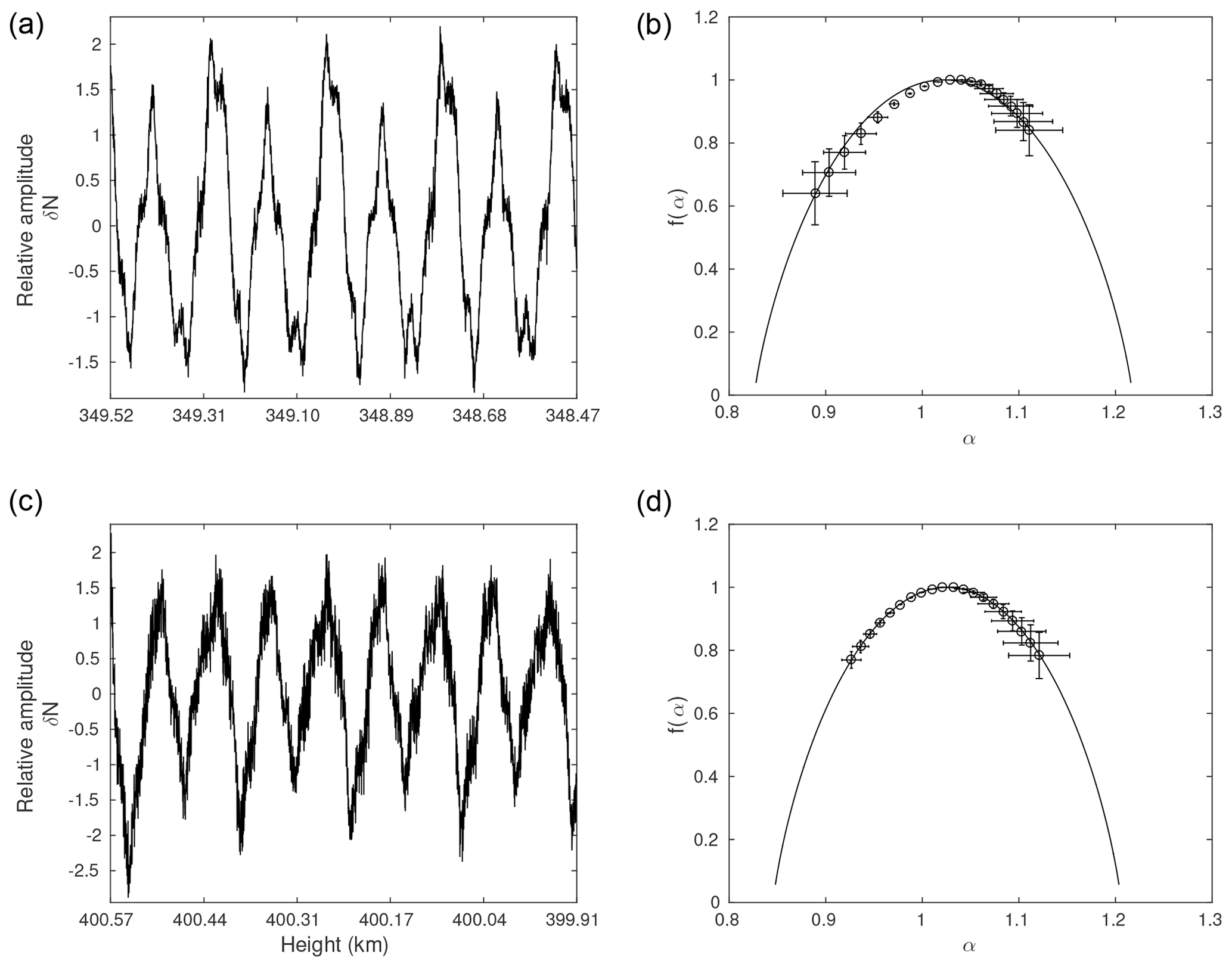
https://www.ann-geophys.net/38/445/2020/angeo-38-445-2020-f04

Figure 4MFDFA for the second experiment: panels (a, b) show the multifractal analysis of the time series at mean height 348.99 km and panels (c, d) show the multifractal analysis of the time series at mean height 400.24 km. Panels (a, c) show the time series for given mean height and panels (b, d) show the multifractal spectrum fitted with the p-model (continuous line).

Download

Figure 1 shows a detailed multifractal analysis of a time series from the first experiment, corresponding to the mean height of 324.00 km (a). The profile of h(q) as a function of q is shown in Fig. 1b, and of τ(q) in 1c. The corresponding multifractal spectrum is shown in Fig. 1d. The spectrum is right-skewed, indicating the influence of the negative values of q on the data. It is evident as well from the h(q) profile that the variation of h(q) for negative q is observed to be comparatively steep. The plot for τ(q) versus q shows marked deviation from the linearity, asserting the presence of the multifractality in the time series for the chosen height. In addition to the derived inferences from the visual analysis of the multifractal spectrum reported above, multifractal measures, Δα, and A can be quantified (Eqs. 11 and 10). Measure A=0.32 quantifies the skewness while Δα=0.72 infers the strength of multifractality. These two measures are listed in Table 1. Lastly, the multifractal spectrum is fitted with the p-model (shown with a continuous line), where the fragment lengths are equal; i.e., $l_{1} = l_{2} = 0.5$ and the weights, p₁ and p₂, are varied such that $p_{1} + p_{2} \leq 1$ . Nevertheless, the loss in p parameter had to be accounted for to obtain an optimal fit. The loss factor, dp, signifies nonconservative energy distribution, i.e., a dissipative energy cascading process in the inertial range. We have obtained a dissipative factor of 0.090, with p₁=0.315. The p-model fit parameters are listed in Table 1.

Similar to Fig. 1, Fig. 2 shows a detailed multifractal analysis of a time series from the second experiment, corresponding to the mean height of 339.94 km (a). The profile of h(q) as a function of q is shown in Fig. 2b, and of τ(q) in Fig. 2c. The corresponding multifractal spectrum is shown in Fig. 2d. The spectrum is left-skewed, indicating the influence of the positive values of q on the data. The variation of h(q) for positive q is observed to be comparatively steep. The plot for τ(q) versus q show a marked deviation from the linearity, asserting the presence of the multifractality in the time series for the chosen height. The multifractal measures computed, A=1.34 and Δα=0.27, and listed in Table 2. Lastly, the multifractal spectrum is fitted with the p-model (shown with a continuous line). We have obtained a dissipative factor of 0.012, with p₁=0.423. The p-model fit parameters are listed in Table 2.

It is seen from the above description that the multifractal spectrum is sufficient to assess the multifractal nature; henceforth we show the time series and the corresponding multifractal spectrum for the remaining chosen heights.

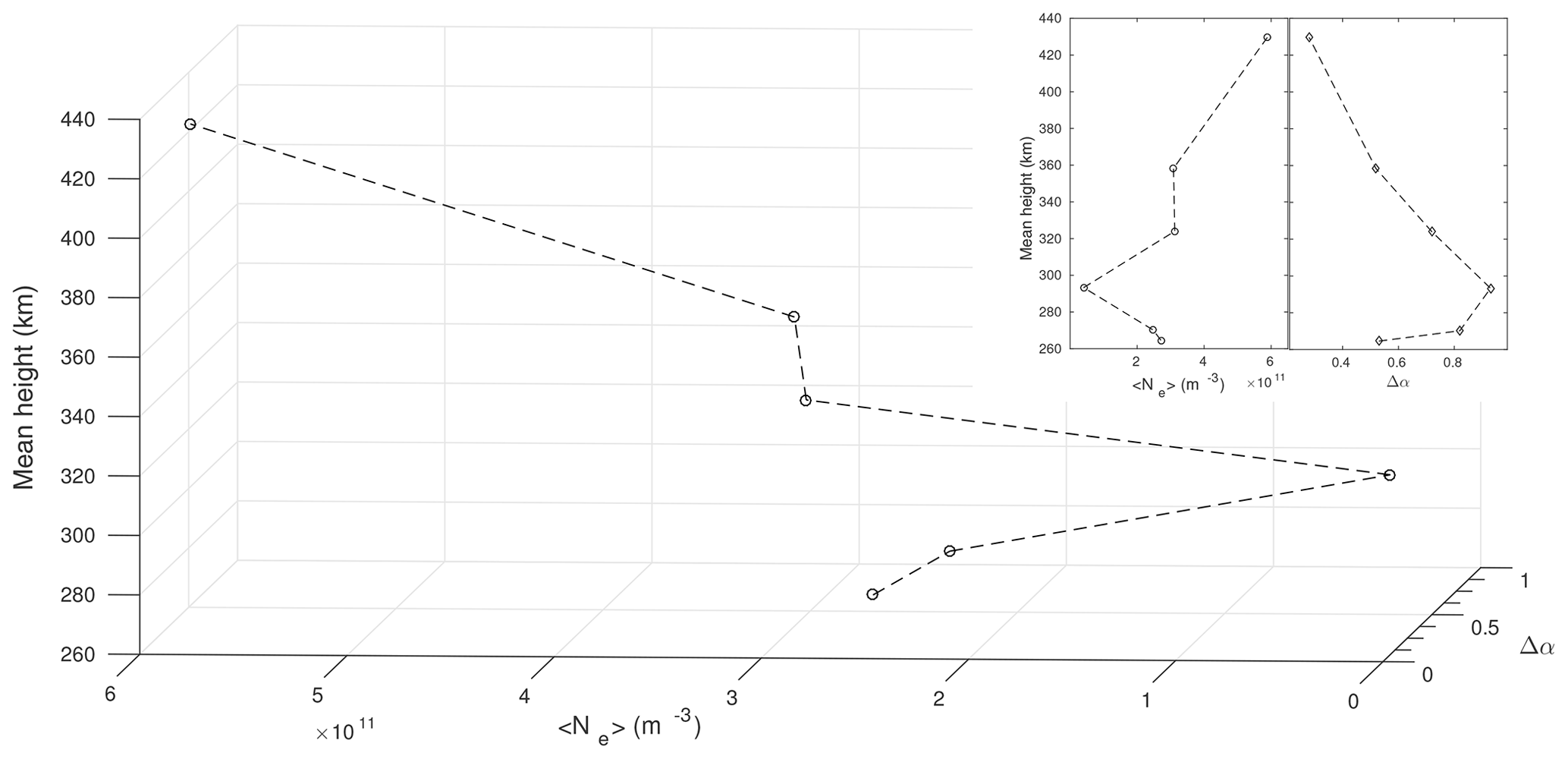
https://www.ann-geophys.net/38/445/2020/angeo-38-445-2020-f05

Figure 5Variation of the mean density and the degree of multifractality with the mean height for the six selected time series from the first experiment in a 3-D plane. These variations are shown in a 2-D plane of the mean density (main image) and the degree of multifractality (inset).

Download

Figure 3 shows the time series selected from the first experiment in the left panels and the corresponding multifractal spectrum in the right panels:

For the time series corresponding to the mean height of 264.58 km, the multifractal spectrum is slightly right-skewed, which can be inferred from measure A=0.82. It indicates the influence of negative moments, q, which characterizes the influence of smaller fluctuations than the average. The degree of multifractality is Δα=0.53. The optimal p-model fit is obtained with parameters p₁=0.364 and dp=0.059.
For the time series corresponding to the mean height of 270.22 km, the multifractal spectrum is slightly left-skewed, which can be inferred from measure A=1.11. It indicates the influence of positive moments, q, which characterize intense larger fluctuations than the average. The degree of multifractality is Δα=0.82. The optimal p-model fit is obtained with parameters p₁=0.34 and dp=0.065.
For the time series corresponding to the mean height of 292.37 km, the multifractal spectrum is left-skewed, reflected in measure A=2.99. It indicates the influence of positive moments, q, which characterize intense larger fluctuations than the average. The degree of multifractality is Δα=0.93. The optimal p-model fit is obtained with parameters p₁=0.339 and dp=0.02. We could fit the spectrum corresponding to positive values of q.
For the time series corresponding to the mean height of 358.56 km, the multifractal spectrum is right-skewed, reflected in measure A=0.37. It indicates the influence of negative moments, q, which characterize the influence of smaller fluctuations than the average. The degree of multifractality is Δα=0.52. The optimal p-model fit is obtained with parameters p₁=0.36 and dp=0.07.
For the time series corresponding to the mean height of 429.65 km, the multifractal spectrum is right-skewed, also reflected in measure A=0.51. It indicates the influence of negative moments, q, which characterize the influence of smaller fluctuations than the average. Degree of multifractality is Δα=0.28. The optimal p-model fit is obtained with parameters p₁=0.399 and dp=0.0355.

Figure 4 shows the time series selected from the second experiment in Fig 4a and c and the corresponding multifractal spectrum in Fig 4b and d:

For the time series corresponding to the mean height of 348.99 km, the multifractal spectrum is left-skewed, reflected in measure A=1.72. It indicates the influence of positive moments, q, which characterize intense larger fluctuations than the average. The degree of multifractality is Δα=0.22. The optimal p-model fit is obtained with parameters p₁=0.43 and dp=0.006.
For the time series corresponding to the mean height of 400.24 km, the multifractal spectrum is almost symmetrical. This is reflected in measure A=0.94, which is very close to 1. It indicates that both negative and positive moments of q characterize the influence of larger and smaller fluctuations than the average almost equally. The degree of multifractality is Δα=0.19. The optimal p-model fit is obtained with parameters p₁=0.4335 and dp=0.01.

Figure 5 shows a variation of mean density and multifractal width, Δα, with mean heights for the selected six time series on a three-dimensional plane. The presence of a plasma bubble characterized by large-scale irregularities, which in turn is reflected in the low density, is observed around a mean height of 292.37 km. Contrarily, stronger multifractality is observed at this height. This inverse variation is in agreement with the turbulent-seeming multiplicative cascade process. On the other hand, as the rocket traversed higher altitudes, the mean density increased while the multifractality became weaker. This suggests that the cascading process resulted in smaller-scale irregularities due to dissipating energy. Two-dimensional plots showing the variation of mean density and Δα with mean heights are shown in Fig. 5.

5 Concluding remarks

In this work, we investigate the in situ F region electric field and electron density measurements obtained from the two experiments carried out near the equatorial sites in Brazil using the MFDFA to understand the complexity in the data and to identify the signature of multiplicative energy cascades in irregularities.

In all the time series, we obtained $0.9 < h (q) < 1.5$ , which indicates a long-range correlation with persistent temporal fluctuations. In addition, we note that the h(q) profile monotonically decreases with respect to q and that τ(q) shows deviation from the linearity, indicating the presence of the multifractality in all time series. Measures of multifractal spectra, A, have shown the presence of structures (both smaller or larger) in the fluctuations, and Δα has shown weaker to stronger multifractality. The multifractal spectra were fitted with the p-model and we found weight parameter p₁ to be different from 0.5, which confirms the multifractality present in the data. The accounting nonzero dissipation factor suggests that energy distribution across the eddies is nonuniform. Our results show the nonhomogenous and intermittent nature of ionospheric irregularities are consistent with previous findings.

In the second experiment, we considered a total of six time series, out of which three time series exhibited a monofractal nature, and the remaining three showed weaker multifractality and are presented here. Δα and skewness are found to be smaller compared to the first experiment. The result for a mean height of 348.99 km is different than for the other two heights and shows evidence of some different kind of physical mechanism, which can be described by the multiplicative cascade process. Though time series are characterized by weaker multifractality, these data have fractal behavior with long-range correlation. However, we argue that more detailed study is required to reach any definite conclusion on the turbulent-seeming mechanism driving the ionospheric irregular structures.

Finally, we intend to test the potential of this algorithm in deciphering the morphology of the cascading phenomena. For this, we choose the first experiment where the rocket intercepted a plasma bubble. Muralikrishna et al. (2003) reported the presence of predominant sharp peaks in the power spectra over a wide range of heights, and they attribute these to a developing plasma bubble that subsequently dissipated energy, reaching an equilibrium which is evidenced by the absence of peaks. Our multifractal analysis has captured this sequence of events.

The presence of a plasma bubble characterized by large-scale irregularities, which in turn is reflected in the low density, is observed around a mean height of 292.37 km. Contrarily, stronger multifractality is observed at this height. This inverse variation is in agreement with the turbulent-seeming multiplicative cascade process. On the other hand, as the rocket traversed higher altitudes, the mean density increased while the multifractality became weaker. This suggests that the cascading process resulted in smaller-scale irregularities by dissipating energy.

We conclude at this point where we have presented the schematic hypothesis based on the multifractal analysis of plasma irregularities in the ionospheric F region.

Data availability

The data used in this analysis are available at the National Institute for Space Research library archive through, available at: http://urlib.net/rep/8JMKD3MGP3W34R/803U8PQA8 (last access: 17 October 2019, INPE, 2019).

Author contributions

All authors have contributed to the analysis and development of the manuscript.

Competing interests

The authors declare that they have no conflict of interest.

Special issue statement

This article is part of the special issue “7th Brazilian meeting on space geophysics and aeronomy”. It is a result of the Brazilian meeting on Space Geophysics and Aeronomy, Santa Maria/RS, Brazil, 5–9 November 2018.

Acknowledgements

The authors are thankful to the Institute of Aeronautics and Space (IAE/DCTA) and Alcântara Launch Center (CLA) for providing sounding rockets and for the launch operation, respectively. Also, we are grateful to Abraham L. Chian for his constructive comments and review on PSD-based ionospheric studies, which has been adopted in this article, and to another anonymous reviewer for his or her comments that have increased the clarity of the article. Neelakshi Joshi thanks CAPES for supporting her PhD and is grateful to Anna Wawrzaszek for the discussion and guidance obtained on the multifractal analysis and p-model. RRR acknowledges FAPESP grant no. 14/11156-4. Siomel Savio acknowledges the financial support from the Chinese–Brazilian Joint Laboratory for Space Weather, the National Space Science Center, and the Chinese Academy of Science. Francisco Carlos de Meneses is grateful to the financial support provided by the National Council of Science and Technology of Mexico (CONACYT), the CAS-TWAS Fellowship for Postdoctoral and Visiting Scholars from Developing Countries (201377GB0001), and the Brazilian Council for Scientific and Technological Development (CNPq), grants 312704/2015-1 and 313569/2019-3.

Financial support

This research was mostly supported through the CAPES scholarship for the PhD program in applied computing at INPE (grant no. 0028-15/2015). We hereby certify that this grant was active from March 2015 to February 2019.

Review statement

This paper was edited by Igo Paulino and reviewed by Abraham C. L. Chian and one anonymous referee.

References

Abdu, M. A., Nogueira, P. A. B., Santos, A. M., de Souza, J. R., Batista, I. S., and Sobral, J. H. A.: Impact of disturbance electric fields in the evening on prereversal vertical drift and spread F developments in the equatorial ionosphere, Ann. Geophys., 36, 609–620, https://doi.org/10.5194/angeo-36-609-2018, 2018. a

Abramenko, V. I., Yurchyshyn, V. B., Wang, H., Spirock, T. J., and Goode, P. R.: Scaling behavior of structure functions of the longitudinal magnetic field in active regions of the Sun, Astrophys. J., 577, 487–495, https://doi.org/10.1086/342169, 2002. a

Alimov, V. A., Vybornov, F. I., and Rakhlin, A. V.: Multifractal Structure of Intermittency in a Developed Ionospheric Turbulence, Radiophys. Quantum. El., 51, 438, https://doi.org/10.1007/s11141-008-9044-4, 2008. a

Bolzan, M. J. A., Tardelli, A., Pillat, V. G., Fagundes, P. R., and Rosa, R. R.: Multifractal analysis of vertical total electron content (VTEC) at equatorial region and low latitude, during low solar activity, Ann. Geophys., 31, 127–133, https://doi.org/10.5194/angeo-31-127-2013, 2013. a, b

Cander, L. R.: Ionospheric Space Weather Targets, in: Ionospheric Space Weather, Springer International Publishing, 245–264, https://doi.org/10.1007/978-3-319-99331-7_9, 2019. a

Carbone, V., Bruno, R., and Veltri, P.: Scaling laws in the solar wind turbulence, in: Small-Scale Structures in Three-Dimensional Hydrodynamic and Magnetohydrodynamic Turbulence, edited by: Meneguzzi, M., Pouquet, A., and Sulem, P. L., Lect. Notes Phys., 462, 153–158, https://doi.org/10.1007/BFb0102411, 1995. a

Chandrasekhar, E., Prabhudesai, S. S., Seemala, G. K., and Shenvi, N.: Multifractal detrended fluctuation analysis of ionospheric total electron content data during solar minimum and maximum, J. Atmos. Sol.-Terr. Phy., 149, 31–39, https://doi.org/10.1016/j.jastp.2016.09.007, 2016. a, b

Chian, A. C.-L. and Muñoz, P. R.: Detection of current sheets and magnetic reconnections at the turbulent leading edge of an interplanetary coronal mass ejection, Astrophys. J. Lett., 733, L34, https://doi.org/10.1088/2041-8205/733/2/l34, 2011. a

Chian, A. C.-L., Abalde, J. R., Miranda, R. A., Borotto, F. A., Hysell, D. L., Rempel, E. L., and Ruffolo, D.: Multi-spectral optical imaging of the spatiotemporal dynamics of ionospheric intermittent turbulence, Sci. Rep., 8, 10568, doi:10.1038/s41598-018-28780-5, 2018. a

Costa, E. and Kelley, M. C.: On the role of steepened structures and drift waves in equatorial spread F, J. Geophys. Res., 83, 4359–4364, https://doi.org/10.1029/JA083iA09p04359, 1978. a

de Freitas, D. B., Nepomuceno, M. M. F., de Moraes Junior, P. R. V., Lopes, C. E. F., Das Chagas, M. L., Bravo, J. P., Costa, A. D., Canto Martins, B. L., De Medeiros, J. R., and Leão, I. C.: New suns in the cosmos, III. Multifractal signature analysis, Astrophys. J., 831, 87, https://doi.org/10.3847/0004-637x/831/1/87, 2016. a

Dyrud, L., Krane, B., Oppenheim, M., P/'ecseli, H. L., Trulsen, J., and Wernik, A. W.: Structure functions and intermittency in ionospheric plasma turbulence, Nonlinear Proc. Geoph., 15, 847–862, 2008. a

Fornari, G., Rosa, R., De Meneses, F. C., and Muralikrishna, P.: Spectral fluctuation analysis of ionospheric inhomogeneities over Brazilian territory, Part I: Equatorial F-region plasma bubbles, Adv. Space Res., 58, 2037–2042, https://doi.org/10.1016/j.asr.2016.03.039, 2016. a

Grauer, R., Krug, J., and Marliani, C.: Scaling of high-order structure functions in magnetohydrodynamic turbulence, Phys. Lett. A, 195, 335–338, https://doi.org/10.1016/0375-9601(94)90038-8, 1994. a

Grech, D.: Alternative measure of multifractal content and its application in finance, Chaos. Soliton. Fract., 88, 183–195, https://doi.org/10.1016/j.chaos.2016.02.017, 2016 a

Halsey, T., Jensen, M., Kadanoff, L., Procaccial, I., and Shraiman, B.: Fractal measures and their singularities: The characterization of strange sets, Phys. Rev. A, 33, 1141–1151, 1986. a, b

Hysell, D. L., Kelley, M. C., Swartz, W. E., Pfaff, R. F., and Swenson, C. M.: Steepened structures in equatorial spread F: 1. New observations, J. Geophys. Res., 99, 8827–8840, https://doi.org/10.1029/93JA02961, 1994. a

Hysell, D. L., Seyler, C. E., and Kelley, M. C.: Steepened structures in equatorial spread F: 2. Theory, J. Geophys. Res., 99, 8841–8850, https://doi.org/10.1029/93JA02960, 1994. a

Ihlen Espen: Introduction to Multifractal Detrended Fluctuation Analysis in Matlab, Front. Physiol., 3, 141, https://doi.org/10.3389/fphys.2012.00141, 2012. a, b

Biblioteca, National Institute for Space Research (INPE): Structural characterization of the equatorial F region plasma irregularities in the multifractal context, available at: http://urlib.net/rep/8JMKD3MGP3W34R/803U8PQA8 last access: 17 October 2019. a

Jahn, J. M. and LaBelle, J.: Rocket measurements of high-altitude spread F irregularities at the magnetic dip equator, J. Geophys. Res.-Space, 103, 23427–23441, https://doi.org/10.1029/97JA02636, 1998. a, b

Kantelhardt, J., Zschiegner, S., Koscielny-Bunde, E., Havlin, S., Bunde, A., and Stanley, H.: Multifractal detrended fluctuation analysis of nonstationary time series, Physica A, 316, 87–114, 2002. a, b, c

Kantelhardt, J. W. and Meyers, R. A. (Eds.): Fractal and multifractal time series, Encyclopedia of complexity and systems science, Springer New York, 3754–3779, https://doi.org/10.1007/978-0-387-30440-3_221, 2009. a

Kelley, M. C., Seyler, C. E., and Zargham, S.: Collisional interchange instability: 2. A comparison of the numerical simulations with the in situ experimental data, J. Geophys. Res., 92, 10089–10094, https://doi.org/10.1029/JA092iA09p10089, 1987. a

Kelley, M. C. and Hysell, D. L.: Equatorial Spread-F and neutral atmospheric turbulence: A review and a comparative anatomy, J. Atmos. Terr. Phys., 53, 695–708 https://doi.org/10.1016/0021-9169(91)90122-N, 1991. a

Kelley, M. C., Ilma, R. R., and Crowley, G.: On the origin of pre-reversal enhancement of the zonal equatorial electric field, Ann. Geophys., 27, 2053–2056, https://doi.org/10.5194/angeo-27-2053-2009, 2009. a

Li, G., Ning, B., Liu, L., Ren, Z., Lei, J., and Su, S.-Y.: The correlation of longitudinal/seasonal variations of evening equatorial pre-reversal drift and of plasma bubbles, Ann. Geophys., 25, 2571–2578, https://doi.org/10.5194/angeo-25-2571-2007, 2007. a

Lu, X., Zhao, H., Lin, H., and Wu, Q.: Multifractal Analysis for Soft Fault Feature Extraction of Nonlinear Analog Circuits, Math. Probl. Eng., 2016, 7305702, https://doi.org/10.1155/2016/7305702, 2016. a

Macek, W. M.: Multifractality and intermittency in the solar wind, Nonlinear Proc. Geoph., 14, 695–700, 2007. a

Makowiec, D., Rynkiewicz, A., Gałaska, R., Wdowczyk-Szulc, J., and Żarczyńska-Buchowiecka, M.: Reading multifractal spectra: Aging by multifractal analysis of heart rate, Europhys. Lett., 94, 68005, https://doi.org/10.1209/0295-5075/94/68005, 2011. a

Meneveau, C. and Sreenivasan, K.: Simple multifractal cascade model for fully developed turbulence, Phys. Rev. Lett., 59, 1424–1427, 1987. a, b

Miranda, R. A., Chian, A. C.-L., and Rempel, E. L.: Universal scaling laws for fully-developed magnetic field turbulence near and far upstream of the Earth’s bow shock, Adv. Space Res., 51, 1893, https://doi.org/10.1016/j.asr.2012.03.007, 2013. a

Miriyala, S., Koppireddi, P. R., and Chanamallu, S. R.: Robust detection of ionospheric scintillations using MF-DFA technique, Earth Planets Space, 67, 98, https://doi.org/10.1186/s40623-015-0268-1, 2015. a, b

Muralikrishna, P., Vieira, L. P., and Abdu, M. A.: Electron density and electric field fluctuations associated with developing plasma bubbles, J. Atmos. Sol.-Terr. Phy., 65, 1315–1327, https://doi.org/10.1016/j.jastp.2003.08.010, 2003. a, b, c, d, e, f

Muralikrishna, P. and Abdu, M. A.: Rocket measurements of ionospheric electron density from Brazil in the last two decades, Adv. Space Res., 37, 1091–1096, https://doi.org/10.1016/j.asr.2006.02.006, 2006. a, b, c

Muralikrishna, P. and Vieira, L. P.: Equatorial F-region irregularities generated by the Rayleigh-Taylor instability mechanism: rocket observations from Brazil, Rev. Bras. Geof., 25, 6, https://doi.org/10.1590/S0102-261X2007000600016, 2007. a, b, c

Neelakshi, J., Rosa, R. R., Savio, S., De Meneses, F. C., Stephany, S., Fornari, G., and Muralikrishna, P.: Spectral fluctuation analysis of ionospheric inhomogeneities over Brazilian territory, Part II: E-F valley region plasma instabilities, Adv. Space Res., 64, 1592–1599, https://doi.org/10.1016/j.asr.2019.07.015, 2019. a

Peng, C. K., Buldyrev, S. V., Havlin, S., Simons, M., Stanley, H. E., and Goldberger, A. L.: Mosaic organization of DNA nucleotides, Phys. Rev. E, 49, 1685–1689, https://doi.org/10.1103/PhysRevE.49.1685, 1994. a

Savio, S., Muralikrishna, P., Batista, I. S., and de Meneses, F. C.: Wave structures observed in the equatorial F-region plasma density and temperature during the sunset period, Adv. Space Res., 58, 2043–2051, https://doi.org/10.1016/j.asr.2016.07.026, 2016. a, b, c

Savio Odriozola, S., de Meneses Jr., F. C., Muralikrishna, P., Pimenta, A. A., and Kherani, E. A.: Rocket in situ observation of equatorial plasma irregularities in the region between E and F layers over Brazil, Ann. Geophys., 35, 413–422, https://doi.org/10.5194/angeo-35-413-2017, 2017. a, b, c

Savio, S., Sousasantos, J., Pimenta, A. A., Yang, G., Kherani, E. A., Wang, C., and Liu, Z.: Quasiperiodic rising structures in the E-F valley region below the equatorial plasma bubble: A numerical study, J. Geophys. Res.-Space, 124, 7247–7255, https://doi.org/10.1029/2019JA026620, 2019.

Seuront, L., Schmitt, F., Lagadeuc, Y., Schertzer, D., and Lovejoy, S.: Universal multifractal analysis as a tool to characterize multiscale intermittent patterns: example of phytoplankton distribution in turbulent coastal waters, J. Plankton Res., 21, 877–922, 1999.

Sivavaraprasad, G., Otsuka, Y., Tripathi, N. K., Chowdhary, V. R., Ratnam, D. V., and Khan, M. A.: Spatial and temporal characteristics of ionospheric total electron content over Indian equatorial and low-latitude GNSS stations, Conference on Signal Processing And Communication Engineering Systems (SPACES), Vijayawada, 105–108, https://doi.org/10.1109/SPACES.2018.8316326, 2018. a, b

Spicher, A., Miloch, W. J., Clausen, L. B. N., and Moen, J. I.: Plasma turbulence and coherent structures in the polar cap observed by the ICI-2 sounding rocket, J. Geophys. Res.-Space, 120, 10959–10978, https://doi.org/10.1002/2015JA021634, 2015. a, b

Tanna, H. J. and Pathak, K. N.: Multifractal behaviour of the ionospheric scintillation index time series over an Indian low latitude station Surat, J. Atmos. Sol.-Terr. Phy., 109, 66–74, https://doi.org/10.1016/j.jastp.2014.01.009, 2014. a, b, c

Telesca, L. and Lovallo, M.: Revealing competitive behaviours in music by means of the multifractal detrended fluctuation analysis: application to Bach's Sinfonias, P. Roy. Soc. A-Math. Phy., 467, 3022–3032, https://doi.org/10.1098/rspa.2011.0118, 2011. a

Wawrzaszek, A. and Macek, W. M.: Observation of the multifractal spectrum in solar wind turbulence by Ulysses at high latitudes, J. Geophys. Res., 115, A07104, doi:10.1029/2009JA015176, 2010. a

Wawrzaszek, A., Echim, M. and Bruno, R.: Multifractal Analysis of Heliospheric Magnetic Field Fluctuations Observed by Ulysses, Astrophys. J., 876, 153, https://doi.org/10.3847/1538-4357/ab1750, 2019. a

Wernik, A. W., Secan, J. A., and Fremouw, E. J.: Ionospheric irregularities and scintillation, Adv. Space Res., 31, 971–981, https://doi.org/10.1016/S0273-1177(02)00795-0, 2003. a, b, c, d

Zargham, S. and Seyler, C. E.: Collisional interchange instability: 1. Numerical simulations of intermediate‐scale irregularities, J. Geophys. Res., 92, 10073–10088, https://doi.org/10.1029/JA092iA09p10073, 1987. a