the Creative Commons Attribution 4.0 License.
the Creative Commons Attribution 4.0 License.
 | 25 Feb 2020
Plasma transport into the duskside magnetopause caused by Kelvin–Helmholtz vortices in response to the northward turning of the interplanetary magnetic field observed by THEMIS
George K. Parks
Chun Lin Cai
James P. McFadden
Yong Ren
A train of likely Kelvin–Helmholtz (K–H) vortices with plasma transport across the magnetopause has been observed by the Time History of Events and Macroscale Interactions during Substorms (THEMIS) at the duskside of the magnetopause. This unique event occurs when the interplanetary magnetic field (IMF) abruptly turns northward, which is the immediate change to facilitate the K–H instability. Two THEMIS spacecraft, TH-A and TH-E, separated by 3 RE, periodically encountered the duskside magnetopause and the low-latitude boundary layer (LLBL) with a period of 2 min and tailward propagation of 212 km s−1. Despite surface waves also explaining some of the observations, the rotations in the bulk velocity observation, a distorted magnetopause with plasma parameter fluctuations and the magnetic field perturbations, as well as a high-velocity low-density feature indicate the possible formation of rolled-up K–H vortices at the duskside of the magnetopause. The coexistence of magnetosheath ions with magnetospheric ions and enhanced energy flux of hot electrons is identified in the K–H vortices. These transport regions appear more periodic at the upstream spacecraft and more dispersive at the downstream location, indicating significant transport can occur and evolve during the tailward propagation of the K–H waves. There is still much work to do to fully understand the Kelvin–Helmholtz mechanism. The observations of the direct response to the northward turning of the IMF, the possible evidence of plasma transport within the vortices, involving both ion and electron fluxes, can provide additional clues as to the K–H mechanism.
- Article
(7546 KB) - Full-text XML
- BibTeX
- EndNote


Kelvin–Helmholtz (K–H) instability can be activated at the interface between different plasma regimes with different velocities, and the perturbations propagate along the direction of the velocity shear as a form of surface wave developing into nonlinear vortices. As shown by Hasegawa (1975), the high density and the magnetic field perpendicular to the velocity shear on either side of the interface facilitate the unstable condition. The fastest K–H instability occurs when the wave vector k is parallel/antiparallel to the velocity shear and perpendicular to the magnetic field (Southwood, 1979; Manuel and Samson, 1993). This condition favors the low-latitude magnetopause where the velocity shear and the northward magnetospheric magnetic field are available. The magnetic tension stabilizes the shear layer if the magnetic field and the velocity shear are aligned, indicating that the radial interplanetary magnetic field (IMF) does not favor the K–H instability. However, reported observation indicates that K–H waves occur at the high-latitude magnetopause under the dawnward IMF and continue to exist when the IMF turns radial (Hwang et al., 2012). On the other hand, under the radial IMF, K–H instability is found in both simulations (Tang et al., 2013; Adamson et al., 2016) and observations (Farrugia et al., 2014; Grygorov et al., 2016). In some cases, the K–H instability is thought to be facilitated by a denser boundary layer formed by the dayside magnetic reconnections (Grygorov et al., 2016), by the plasma plume (Walsh et al., 2015), or by the pre-existing denser boundary layer formed by the high-latitude reconnections under the northward IMF (Hasegawa et al., 2009; Nakamura et al., 2017). Theoretically, both northward and southward IMF can favor the K–H instability at the low-latitude magnetopause. In fact, almost all of the previous observations (Chen and Kivelson, 1993; Kivelson and Chen, 1995; Fujimoto et al., 2003; Hasegawa et al., 2004) and simulations (Chen et al., 1997; Farrugia et al., 2003; Miura, 1995; Hashimoto and Fujimoto, 2005) show that the K–H waves occur preferentially under the northward IMF, although linear K–H waves are observed under the southward IMF (Mozer et al., 1994; Kawano et al., 1994). However, under the southward IMF, Cluster has observed nonlinear K–H waves with irregular and turbulent characteristics (Hwang et al., 2011), and THEMIS has observed regular K–H vortices with an induced electric field at the edges (Yan et al., 2014). As reviewed (Johnson et al., 2014; Masson and Nykyri, 2016) recently, observations from many missions such as Cluster, THEMIS, Wind, or Geotail, as well as simulations, greatly enriched our understanding of the K–H instability and the vortices. Based on long-term observations, a statistical survey indicates that K–H waves are much more ubiquitous than previously thought (Kavosi and Raeder, 2015), which implies the importance of the solar wind plasma transport into the magnetosphere via the K–H vortices.
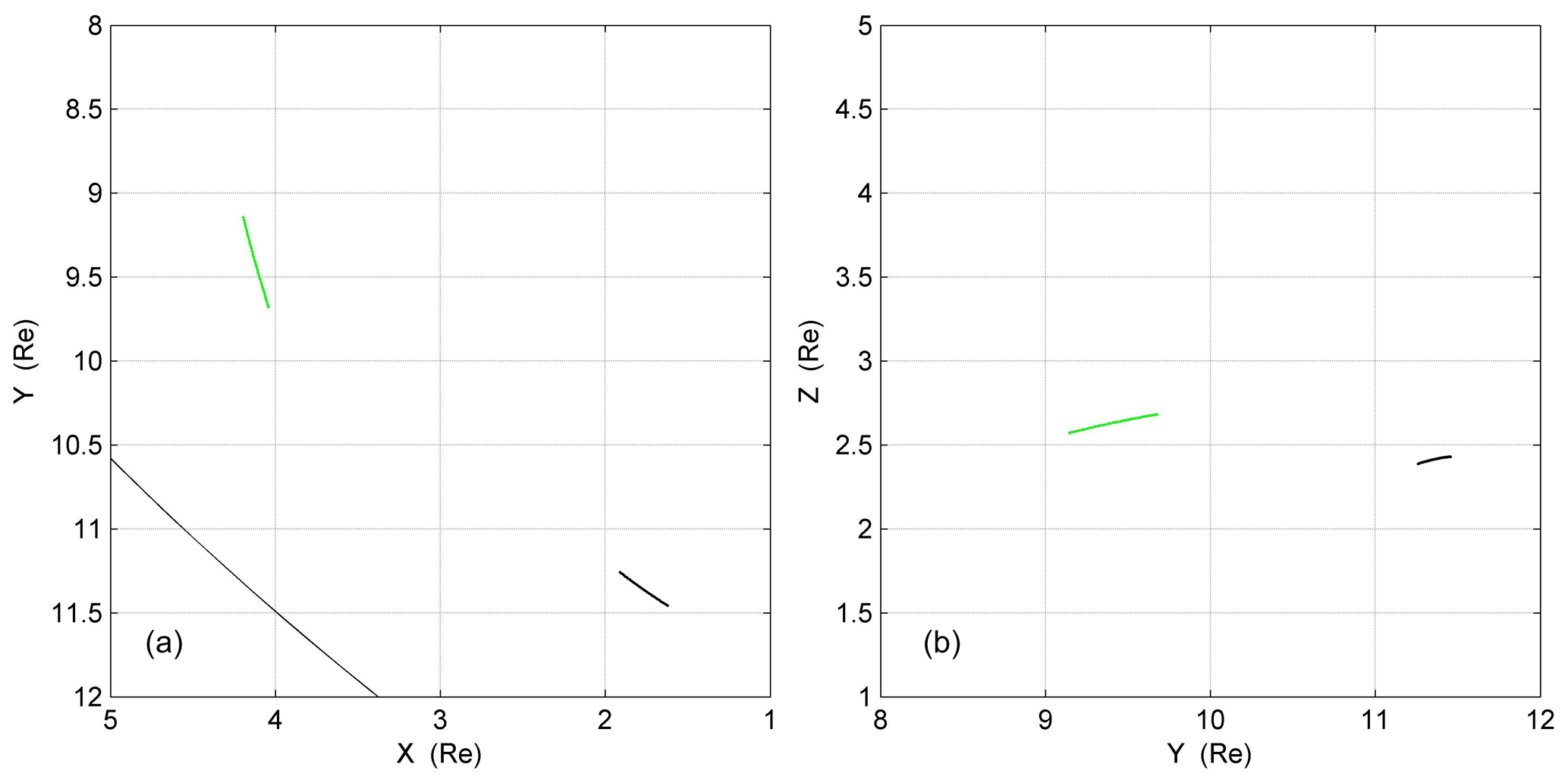
Figure 1The orbits and positions of TH-A (green) and TH-E (black) during the interval of interest 22:20–22:54 UT. The position data are expressed in GSM coordinates.
In addition to magnetic reconnections at the low-latitude (Dungey, 1961) and high-latitude magnetopause (Song and Russell, 1992), whose nature is a popular research topic (e.g., Dai, 2009, 2018; Dai et al., 2017), the K–H instability is an important way to transport solar wind into the magnetosphere when reconnections are inactive at the magnetopause. A statistical study of double star observations implies the entry of cold ions into the flank magnetopause caused by the K–H vortices that is enhanced by solar wind speed (Yan et al., 2005). However, it is noted that the K–H instability itself cannot lead to plasma transport across the magnetopause (Hasegawa et al., 2004); therefore, certain secondary processes (e.g., Nakamura et al., 2004; Matsumoto and Hoshino, 2004; Chaston et al., 2007) are necessarily coupled with the K–H instability for plasma transport into the magnetosphere via the low-latitude boundary layer (LLBL). The reconnection of the twisted magnetic field lines inside the K–H vortex was first found in a simulation (Otto and Fairfield, 2000) and has since been identified in observations (Nykyri et al., 2006; Hasegawa et al., 2009; Li, et al., 2016). The plasma transport into the magnetosphere via such a process in K–H vortices has been quantitatively investigated in a simulation (Nykyri and Otto, 2001). Most recently, energy transport from a K–H wave into a magnetosonic wave was estimated by conserving energy in the cross-scale process, and three possible ways were discussed to transfer energy involving shell-like ion distributions, kinetic Alfvén waves, and magnetic reconnection (Moore et al., 2016). Up to now, there have only been a handful of reports of direct observations of plasma transport in the K–H vortices (e.g., Sckopke et al., 1981; Fujimoto et al., 1998; Hasegawa et al., 2004). Moreover, the microphysical processes for the plasma transport remain unclear, indicating more observations of such a transport process are needed to help us understand the physics. In this work, we present the THEMIS observations of likely K–H vortices activated when the IMF abruptly turns northward. We show a solar wind transport into the magnetosphere occurs and evolves within the vortices.
The THEMIS mission (Angelopoulos, 2008) consists of five identical spacecraft originally orbiting the Earth similarly to a string-of-pearls configuration. In August 2009, TH-B and TH-C were pushed to the vicinity of the lunar orbit, while the other three stayed in the near-Earth orbit with an apogee of approximately 13 RE. The instruments onboard include a flux gate magnetometer (FGM) (Auster et al., 2008) to measure the magnetic field and an electrostatic analyzer (ESA) (McFadden et al., 2008) to measure the electron (6 eV–30 keV) and ion (5 eV–25 keV) fluxes. We used the 3 s averaged FGM and ESA data from TH-A and TH-E to perform the particle analysis and the 1∕16 s averaged FGM data to perform the minimum variance analysis (MVA) (Sonnerup and Cahill, 1967, 1968) to determine the local magnetopause coordinates to find the distortions of the magnetopause. The FGM and ESA data from TH-B located in the dawnside downstream solar wind provide the IMF and solar wind conditions with an estimated time lag of 10 min from the subsolar magnetopause to TH-B. Both ion and electron energy spectra with a 3 s resolution were used to diagnose the transport of the magnetosheath and magnetospheric ions. During the interval of interest, there are no data in the top energy channels centered at 25.21 keV for the ion spectrum and 31.76 keV for the electron spectrum, which has not influenced our investigations.
During the interval 22:20–22:54 UT on 28 March 2016, TH-A and TH-E were located near the magnetopause (Fig. 1), while TH-D was located in the inner magnetosphere, far from the magnetopause. TH-B, near the lunar orbit, was immersed in the solar wind at the dawnside downstream of the other two spacecraft. As shown in panel (a) of Fig. 3, TH-B observed an abrupt turning of the IMF from duskward to northward at 22:32 UT, corresponding to 22:22 UT, with a time lag of 10 min ((10+32.7) RE ∕ (450 km s−1)) from the subsolar magnetopause to TH-B. Periodical fluctuations were observed in both the TH-A and TH-E observations (Fig. 2), from ion density in panel (a), temperature in panel (b), magnetic field in panels (c) and (g), to velocity in panels (d) and (h), especially the alternating appearances of hot and cold ions in the energy–time spectra (panels e and i). The period was approximately 2 min (17 peaks within 34 min), and the tailward bulk propagation speed was approximately 212 km s−1 (3 RE ∕ 90 s). In Fig. 3, the rotational characteristics were identified in the periodical fluctuations in Vl, Vm and Vn with phase differences between them. The magnetic field deviations in panels (c) and (e) indicated the perturbations of the magnetic field along with the deformation of the magnetopause. The alternating appearances of the two different plasmas imply the multiple periodic encounters of the magnetopause and the LLBL, which is one of the typical characteristics of K–H vortices.

Figure 2Fluctuations in the plasma parameters and the ion and electron energy–time spectra. Panel (a) is the ion densities from TH-A as a green line and from TH-E as a black line; panel (b) is the ion temperatures from TH-A as a green line and from TH-E as a black line; panels (c) and (d) are the magnetic field vectors and the ion bulk velocity vectors from TH-A, respectively; panels (e) and (f) are the ion and electron energy–time spectra from TH-A, respectively; panels (g) and (h) are the magnetic field vectors and the ion bulk velocity vectors from TH-E, respectively; panels (i) and (j) are the ion and electron energy–time spectra from TH-E, respectively. Vectors are all expressed in GSM coordinates. The four black arrows mark at the top of panel (e) the TH-A intervals in the magnetosheath. The green bars at the bottom of panel (e) and the black bars at the bottom of panel (i) mark the transport regions in TH-A and TH-E observations, respectively, identified based on the criteria dictated in the text.
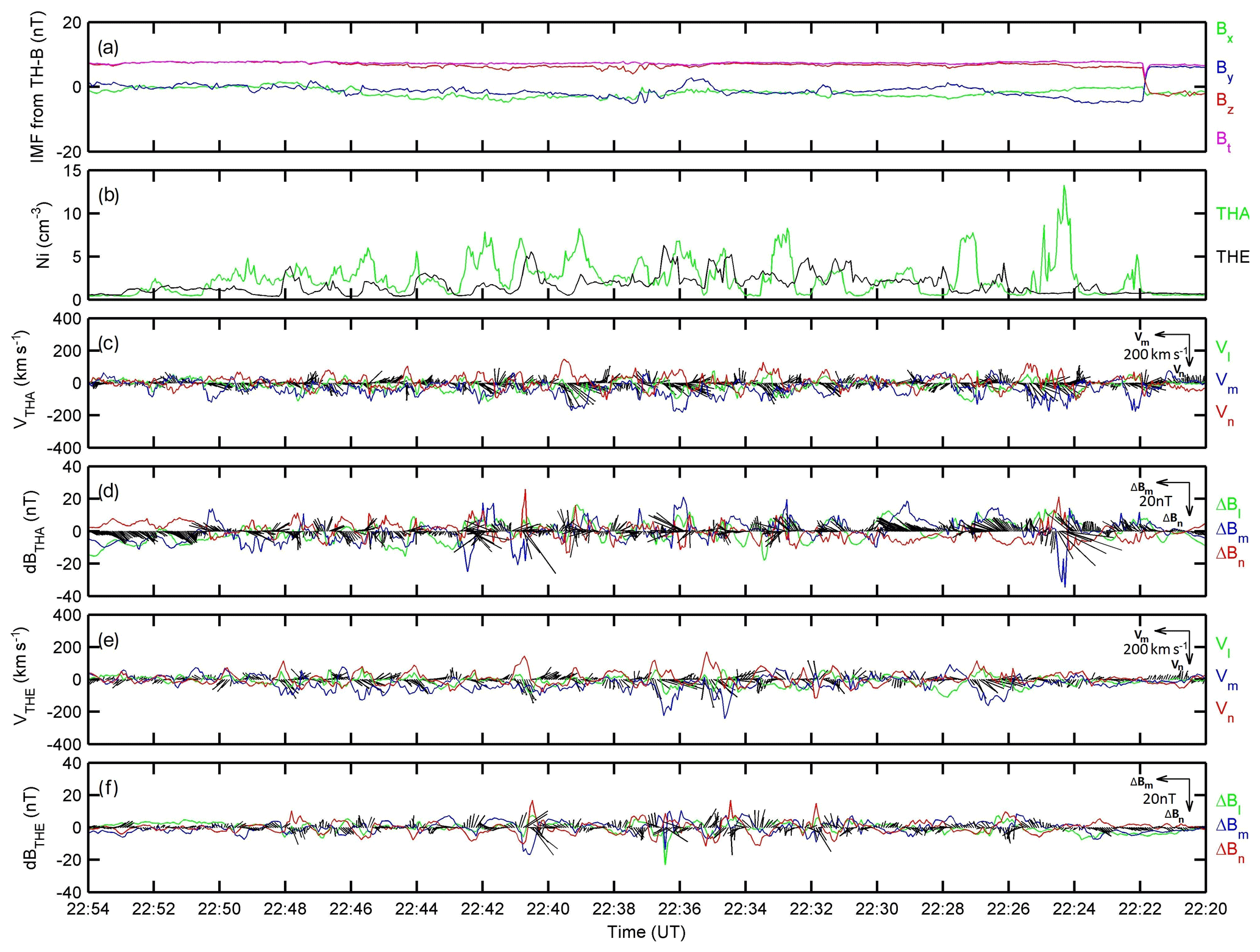
Figure 3The observed plasma rotations and perturbations of the magnetic field because of the formation of K–H vortices. Panel (a) is the IMF monitored by TH-B near the lunar orbit, with a time lag of 10 min from the subsolar magnetopause to TH-B; panel (b) is the ion densities from TH-A in green and from TH-E in black; panels (c) and (e) are the ion bulk velocities from TH-A and TH-E, respectively, expressed in averaged local magnetopause coordinates LMN, deduced from the magnetopause model (Shue et al., 1998); panels (d) and (f) are the magnetic field perturbations, , from TH-A and TH-E, respectively, expressed in LMN. Note that the time begins from the right and passes to the left, so that the M component orients leftward and the N component orients downward in the plots.
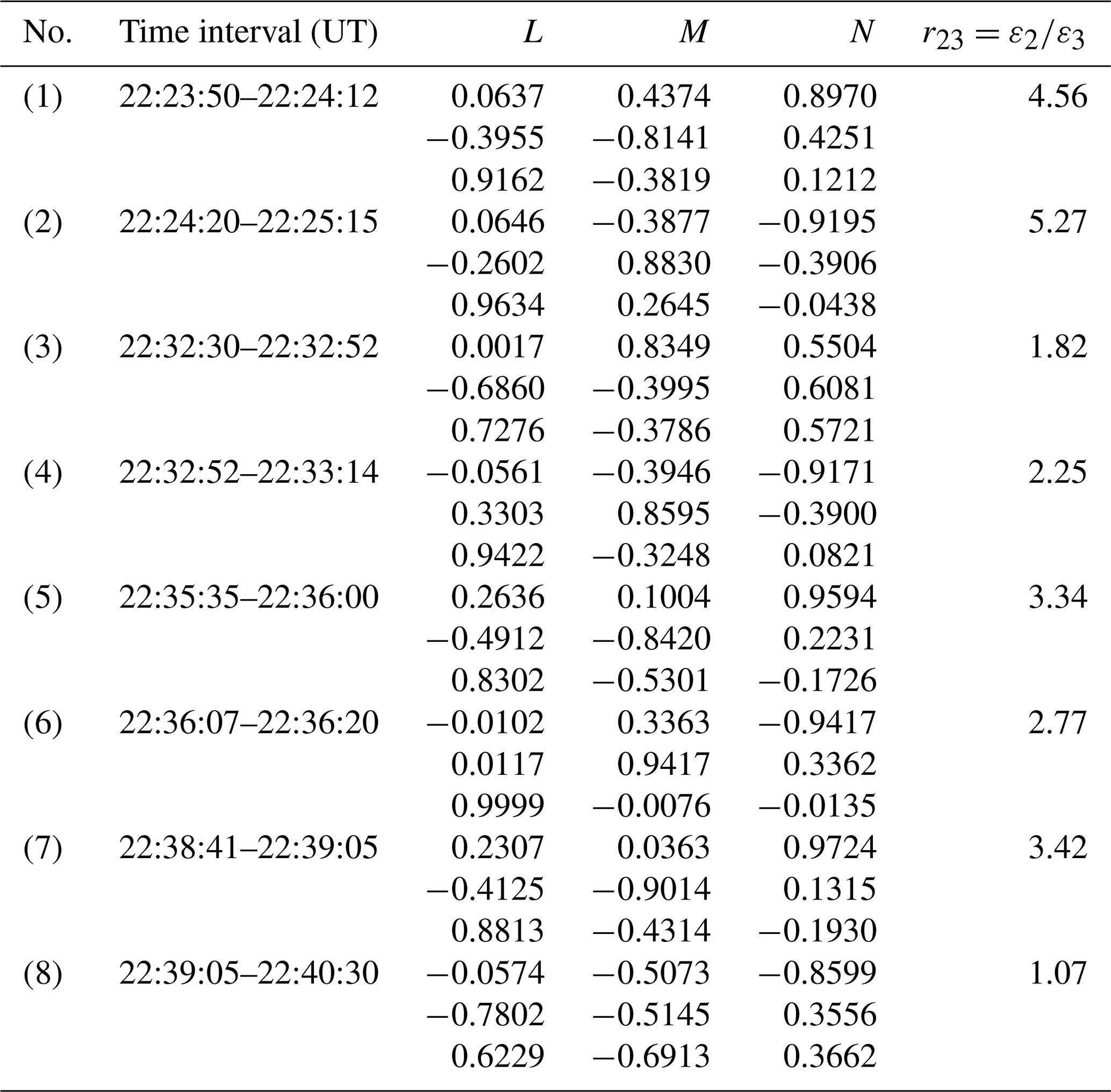
In this event, the IMF is strongly northward, and the observed magnetic field does not change much, so it could be difficult to identify the magnetopause. We selected the four intervals of 22:24:00–22:24:40, 22:32:40–22:33:10, 22:35:50–22:36:10, and 22:28:50–22:39:20 UT, marked by the black arrows, when the TH-A ion spectrum showed the magnetosheath feature. During the four intervals, TH-A observed magnetosheath cold ions without magnetospheric hot ions (green regions at the top of panel e, Fig. 2). The absence of hot ions indicated that the spacecraft had crossed the magnetopause into the magnetosheath, where the outbound and inbound crossings of the magnetopause can be identified in the ion spectrum. At each pair of traversals, the local magnetopause coordinates LMN were calculated by using MVA (Sonnerup and Cahill, 1967, 1968). The details and results of MVA calculations are listed in Table 1. In the calculations of MVA, relatively large ratios of the second to third eigenvalues mean better reliability of determination of local coordinates. In the MVA results, it can be seen that four of eight eigenvalue ratios are larger than 3, indicating the good reliability of the MVA method at their corresponding crossings, even though the magnetic field does not change strongly. At least at these traversals, the magnetopause was deformed into the nonlinear vortices. In some previous research, the threshold of the eigenvalue ratio was taken as 4 (e.g., Sergeev et al., 2006). As for our results, at least, the eigenvalue ratios at the first pair of traversals are larger than 4, which means that the calculated LMN coordinates at the outbound and inbound of the magnetopause are reliable and the magnetopause was deformed into a vortex. The calculated normal direction N as well as the tangential direction M of the local magnetopause are used to identify the distorted magnetopause. In each panel of Fig. 4, the normal and tangential directions M–N at the outbound and inbound magnetopause are plotted in the equatorial plane, compared with the average M–N of the magnetopause. The average magnetopause in dotted line, as well as the average M–N directions, are calculated from the model (Shue, 1998), and the dotted line is also approximately the trajectory of the spacecraft TH-A, which is moving at a relatively slow speed of about 2 km s−1 at the apogee. The distorted magnetopause is plotted in black line, perpendicular to N and parallel to M at outbound and inbound. The deviations of the M–N directions from the averaged magnetopause illustrate the magnetopause distortions formed by the K–H vortices. Such distortions of the magnetopause qualitatively explain the periodically alternating encounters of magnetosphere-like and magnetosheath-like plasmas. The plasma rotation is also illustrated by the red circle with arrow, consistent with the observations in panel (d) of Fig. 2.
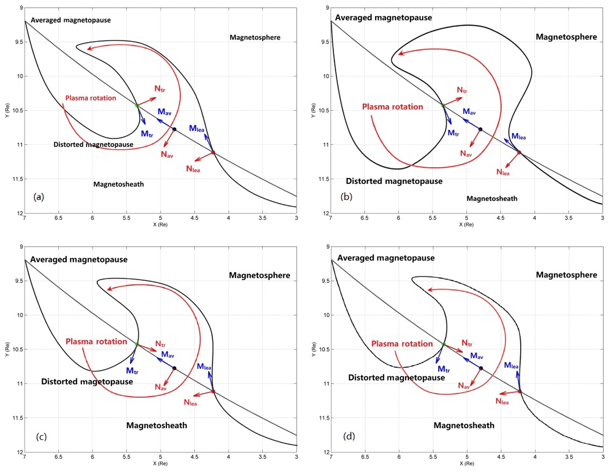
Figure 4The magnetopause distortions formed by the K–H vortices deduced by the MVA. The average magnetopause (dashed lines), approximated to the spacecraft trajectory, was calculated from the magnetopause model (Shue et al., 1998). Traversal pair at 22:24 UT in panel (a): Mlea= (0.4374, −0.8141, −0.3819) and Nlea= (0.8970, 0.4251, 0.1212) at the outbound crossing; Mtr= (−0.3877, 0.8830, 0.2645) and Ntr= (−0.9195, −0.3906, −0.0438) at the inbound crossing. Traversal pair at 22:32 UT in panel (b): Mlea= (0.8349, −0.3995, −0.3786) and Nlea= (0.5504, 0.6081, 0.5721) at the outbound crossing; Mtr= (−0.3946, 0.8595, −0.3248) and Ntr= (−0.9171, −0.3900, 0.0821) at the inbound crossing. Traversal pair at 22:36 UT in panel (c): Mlea= (0.1004, −0.8420, −0.5301) and Nlea= (0.9594, 0.2231, −0.1726) at the outbound crossing; Mtr= (0.3363, 0.9417, −0.0076) and Ntr= (−0.9417, 0.3362, −0.0135) at the inbound crossing. Traversal pair at 22:39 UT in panel (d): Mlea= (0.0363, −0.9014, −0.4314) and Nlea= (0.9724, 0.1315, −0.1930) at the outbound crossing; Mtr= (−0.5073, −0.5145, −0.6913) and Ntr= (−0.8599, 0.3556, 0.3662) at the inbound crossing.
Table 1Results of MVA analysis at the four magnetosheath encounters of TH-A. The ratio of the second to third eigenvalues is shown in the right column.
The high-speed and low-density feature is one of the fundamental characteristics of rolled-up vortices (Nakamura et al., 2004; Takagi et al., 2006) and has been used to identify vortices in single spacecraft measurements (e.g., Hasegawa et al., 2006; Hwang et al., 2011; Grygorov et al., 2016). We estimated the magnetosheath velocity by averaging the TH-A measurements during the four magnetosheath intervals mentioned above, with the magnetosheath velocity of about 134 km s−1. Figure 5 shows the Vm–Ni plot, in which the blue lines mark the high-speed and low-density region. Vm is the tailward velocity, the M component of the measured velocity expressed in the averaged magnetopause coordinates LMN. Substantial data points are distributed in the blue box in Fig. 5, and the high-speed low-density feature can be seen in the Ni–Vm plot. Hence, although the surface waves can also explain some of the observations, the rotations of the plasma flows, the perturbations of the magnetic field, the high-velocity and low-density feature, and the distortions of the magnetopause support the likely formation of rolled-up K–H vortices. However, the low eigenvalue ratios at some traversals of the magnetopause and the uncertainty of estimating the magnetosheath velocity would admittedly degrade the evidence of the K–H vortices. It is worth noting that the magnetopause oscillations started as soon as the IMF turned northward at 22:22 UT, which can facilitate the K–H instability, or else, the surface waves were amplified by the K–H instability.
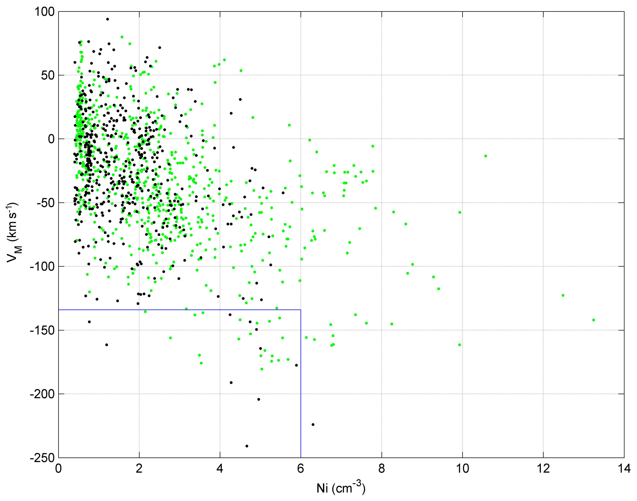
Figure 5The observed velocity along the tailward direction versus the ion density. Green dots are from TH-A observations and black dots from TH-E observations. The blue lines mark the high-speed and low-density region possibly caused by the acceleration of the rotation.
Before and after the 22:22–22:52 UT interval, the magnetospheric hot ions dominated in panel (e) of Fig. 2, mainly in the 3–25 keV range with an energy flux of 106 eV (cm2-s-sr-eV)−1, and the magnetospheric hot electrons dominated in panel (f), mainly in the 0.5–25 keV range with an energy flux of over 107 eV (cm2-s-sr-eV)−1. The typical temperatures of magnetospheric hot ions and electrons were about 4 and 0.3 keV, respectively. On the other hand, during the 22:22–22:52 UT interval, the repeating magnetosheath cold ions in panel (e) were primarily observed between 0.1 and 3 keV with an energy flux of over 106 eV (cm2-s-sr-eV)−1, and the cold electrons in panel (f) were observed between 10 and 500 eV, with an energy flux of over 107 eV (cm2-s-sr-eV)−1. The typical temperatures of magnetosheath cold ions and electrons were about 0.2 and 0.05 keV, respectively. Embedded in the plasmas of the two different origins, the coexisting hot and cold ions overlapped. Taking the mass ratio of protons to electrons into account, the gyro-radius of the electrons is only 1∕42 of protons with the same energy and the same magnetic field, estimated to be approximately 2 km. We understand the ion transport as the coexistence of magnetosheath and magnetospheric ions in the observations, characterized by the substantial cold ions in the steady background of the hot plasma. For the proton's gyro-radius of approximately 80–100 km at the magnetopause, the coexistence of the hot and cold ions in the spectrum is not sufficient to diagnose the mixture of the two components. Thus, we used the observed hot electrons as an additional indicator of the magnetosphere region because of their relatively smaller gyro-radius. Hence, the criteria to identify the coexistence are described such that the cold ions of 0.1–3 keV can be observed with an energy flux over 105 eV (cm2-s-sr-eV)−1 in the hot ion background, with an energy flux over 106 eV (cm2-s-sr-eV)−1, as well as a substantial enhancement in the energy flux of the hot electrons of 0.5–5 keV. Based on such criteria, the ion coexistence intervals were diagnosed from both TH-A and TH-E, marked by the green bars at the bottom of panel (f) and the black bars at the bottom of panel (j) in Fig. 2. The transport regions in the TH-A observations (green bars) were distributed at the edges of the vortices and appeared to be more periodic, while those in the TH-E observations (black bars) were more dispersive. Such an evolution implies the possible plasma transport, although a pre-existing LLBL or the difference of a spacecraft's distances to the magnetopause can also be a potential source.
The coexistence of hot and cold ions is one direct feature of the solar wind transport into the magnetosphere, as clearly displayed in Geotail observations by Fujimoto et al. (1998) and in Cluster observations by Hasegawa et al. (2004). In this event, the coexistence of hot and cold ions was firstly noted near the periodically oscillating magnetopause. Furthermore, we used the enhancement of hot electron flux as an indicator of the magnetosphere and set up the more critical criteria to diagnose the coexistence and hence to display the transport regions, as marked by the green bars at the bottom of panel (f) and the black bars at the bottom of panel (j) in Fig. 2. By comparing the green bars and the black bars, it can be found that the transport regions in TH-A observations appear more periodic and those in TH-E observations more dispersed. The difference between the features of transport regions at upstream TH-A and downstream TH-E implies the plasma transport significantly occurred and evolved during the tailward propagation, along with the collapse of the vortices, leading to a kind of turbulence state, as illustrated in previous simulations (Nakamura et al., 2004; Matsumoto and Hoshino, 2004).
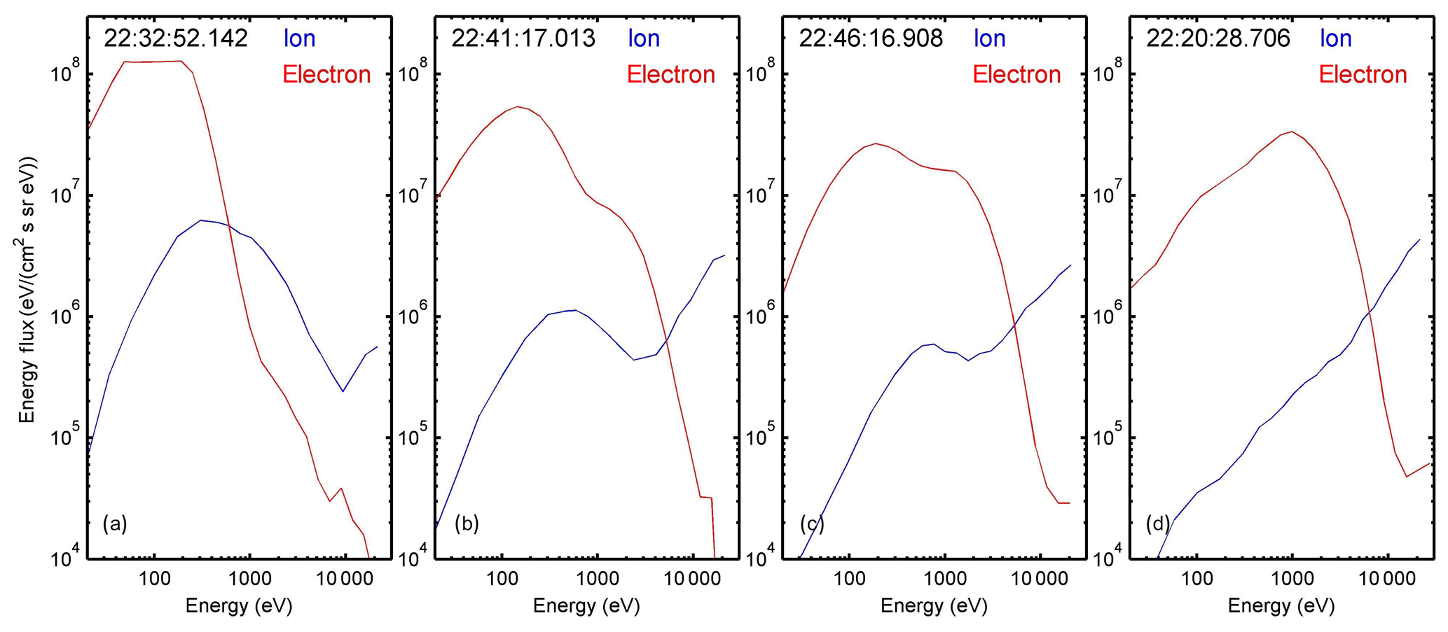
Figure 6Typical portraits of the energy–time spectra of plasmas in different regions. Panel (a) is the magnetosheath observed by TH-A at 22:32:52.142; panel (b) is coexistence region I observed by TH-A at 22:41:17.013; panel (c) is coexistence region II observed by TH-E at 22:46:16.908; panel (d) is the magnetosphere observed by TH-A at 22:20:28.706.
Intuitively, TH-E might be located further inward in the LLBL than TH-A and observed more dispersive oscillations. TH-A observed very clearly periodic motions of the magnetopause during the 34 min except 22:46–22:50 UT and TH-E observed a relatively much more dispersed spectrum during the interval, but five clear oscillations appeared again during 22:40–22:48 UT. However, it seems true that, on the whole, the spectrum observed at TH-E is much more turbulent than the periodic spectrum at TH-A. Such an evolution implies the collapse of the vortices and the evolution leading to a turbulence state. In previous simulations (Nakamura et al., 2004; Matsumoto and Hoshino, 2004), the vortices collapse and cause transport of the solar wind into the magnetosphere; after that, new vortices may be generated at the recovered magnetopause. The five oscillations during 22:40–22:48 UT at downstream TH-E can by explained as newly formed vortices. As mentioned above, the first K–H wave, as well as the transport regions, arrived at the upstream TH-A as soon as the IMF abruptly turned northward. The K–H vortices were evidently activated as a response to the abrupt northward turning of the IMF, which was the direct change to facilitate the K–H instability immediately.
Previously, both electron and ion distributions were used to diagnose the region of observation (Chen et al., 1993). While diagnosing the transport regions in this event, the typical plasma features in different regions were selected for comparisons (Fig. 6), as illustrated by the energy flux distributions of both ions (blue line) and electrons (red line). In panel (a), both the ion and electron fluxes show single peaks at low energy, indicating the components of a cold and dense magnetosheath plasma. In panel (b), the ion flux shows a double peak, which means the coexistence of the magnetosheath cold ions and magnetospheric hot ions. The relatively smaller peak/enhancement in the electron flux shows that the magnetospheric hot electrons are detected, but the cold electrons dominate, implying the spacecraft is located in the magnetosheath but very close to the magnetopause, a coexistence region. In panel (c), both the ion and electron fluxes show a double peak. The double peak of the ion flux indicates the coexistence of the magnetosheath cold ions and magnetospheric hot ions. For the electron flux, the peak at the high energy indicates that more magnetospheric hot electrons are detected, implying that the spacecraft is located in the magnetosphere, another example of a coexistence region. In panel (d), both ion and electron fluxes show single peaks at high energy, indicating the components of hot and tenuous magnetospheric plasma. It should be noted that the ion flux plots (blue lines in each panel) should be lower in the tail, but show no such decrease tails in part because the data were absent at the high-energy channels. The typical regions shown correspond to the magnetosheath, the energetic particle streaming layer, the LLBL, and the magnetosphere (Sibeck, 1991).
We analyzed observations from TH-A and TH-E that periodically encountered the magnetopause and the LLBL. Although they could be possibly caused by surface waves, the periodical encounters, characterized by the rotation features in the bulk velocity, magnetic field deviations, the high-speed low-density features and the distortions of the magnetopause deduced by MVA showed the likely generation of K–H vortices. The K–H vortices started, or else, the surface waves were amplified by the K–H instability as soon as the IMF turned northward abruptly, which is the direct change to facilitate the instability immediately. By considering the enhancement of the hot electrons as an indicator of the magnetosphere region, typical plasma features were observed in different regions such as the energetic particle streaming layer, the LLBL, and the magnetosphere. The evolution between periodic and dispersed magnetopause observations from TH-A to TH-E implied the possible plasma transport, which is consistent with the different features of the coexisting regions of cold and hot plasmas between TH-A and TH-E. These new observations can complement existing observations and enhance our understanding of the plasma transport processes in K–H vortices.
The data for this paper are available at the Coordinated Data Analysis Web of NASA's Goddard Flight Center (https://cdaweb.sci.gsfc.nasa.gov/cgi-bin/eval2.cgi, last access: Goddard Space Flight Center, 2020).
GQY designed the idea, carried out the investigations, and prepared the manuscript with contributions from all the co-authors. GKP, CLC, and TC offered the valuable scientific discussions and helped to improve the manuscript. JPM ensured the data and gave valuable suggestions. YR prepared some of the figures.
The authors declare that they have no conflict of interest.
The authors are grateful to NASA's Goddard Flight Center and the associated instrument teams for supplying the data. The authors thank Chi Wang and Lei Dai for valuable scientific discussions. Part of the work was done during Guang Qing Yan's visit at UC Berkeley, who cordially appreciates the assistance from Forrest S. Mozer.
This research has been supported by the Strategic Pioneer Program on Space Science, the Chinese Academy of Sciences (grant nos. XDA15052500, XDA15350201, and XDA17010301), the National Natural Science Foundation of China (grant nos. 41574161, 41731070, 41574159, and 41004074), the National Space Science Center CAS-NSSC-135 project (grant no. Y92111BA8S), and the Specialized Research Fund for State Key Laboratories.
This paper was edited by Anna Milillo and reviewed by two anonymous referees.
Adamson, E., Nykyri, K., and Otto, A.: The Kevin-Helmholtz instability under Parker-Spiral interplanetary Magnetic Field conditions at the magnetospheric flanks, Adv. Space Res., 58, 218–230, 2016.
Angelopoulos, V.: The THEMIS mission, Space Sci. Rev., 141, 5–34, https://doi.org/10.1007/s11214-008-9336-1, 2008.
Auster, U., Glassmeier, K. H., Magnes, W., Aydogar, O., Baumjohann, W., Constaninescu, D., Fischer, D., Fornicon, K. H., Georgescu, E., Harvey, P., Hillenmaier, O., Kroth, R., Ludlam, M., Narita, Y., Nakamura, R., Okrafca, K., Plaschke, F., Richter, I., Schwartzl, H., Stoll, B., Vanavanoglou, A., and Wiedemann, M.: The THEMIS fluxgate magnetometer, Space Sci. Rev., 141, 235–264, https://doi.org/10.1007/s11214-008-9365-9, 2008.
Chaston, C. C., Wilber, M., Mozer, F. S., Fujimoto, M., Goldstein, M. L., Acuna, M., Rème, H., and Fazakerley, A.: Mode conversion and anomalous transport in Kelvin-Helmholtz vortices and kinetic Alfvén waves at the Earth's magnetopause, Phys. Rev. Lett., 99, 175004, https://doi.org/10.1103/PhysRevLett.99.175004, 2007.
Chen, Q., Otto, A., and Lee, L. C.: Tearing instability, Kelvin-Helmholtz instability, and magnetic reconnection, J. Geophys. Res., 102, 151–161, 1997.
Chen, S. H. and Kivelson, M. G.: On nonsinusoidal waves at the magnetopause, Geophys. Res. Lett., 20, 2699–2702, 1993.
Chen, S.-H., Kivelson, M. G., Gosling, J. T., Walker, R. J., and Lazarus, A. J.: Anomalous aspects of magnetosheath flow and of the shape and oscillations of the magnetopause during an interval of strongly northward interplanetary magnetic field, J. Geophys., 98, 5727–5742, 1993.
Dai, L.: Collisionless Magnetic Reconnection via Alfvén Eigenmodes, Phys. Rev. Lett., 102, 245003, https://doi.org/10.1103/PhysRevLett.102.245003, 2009.
Dai, L.: Structures of Hall Fields in Asymmetric Magnetic Reconnections, J. Geophys. Res.-Space, 123, 7332–7341, https://doi.org/10.1029/2018JA025251, 2018.
Dai, L., Wang, C., Zhang, Y., Lavraud, B., Burch, J., Pollock, C., and Torbert, R. B.: Kinetic Alfvén wave explanation of the Hall fields in magnetic reconnection, Geophys. Res. Lett., 44, 634–640, https://doi.org/10.1002/2016GL071044, 2017.
Dungey, J. W.: Interplanetary magnetic field and auroral zones, Phys. Rev. Lett., 6, 47–48, 1961.
Farrugia, C. J., Gratton, F. T., Gnavi, G., Torbert, R. B., and Wilson, L. B.: A vortical dawn flank boundary layer for near-radial IMF: Wind observations on 24 October 2001, J. Geophys. Res.-Space, 119, 4572–4590, https://doi.org/10.1002/2013JA019578, 2014.
Fujimoto, M., Terasawa, T., Mukai, T., Saito, Y., Yamamoto, T., and Kokubun, S.: Plasma entry from the flanks of the near-Earth magnetotail: Geotail observations, J. Geophys. Res., 103, 4391–4408, 1998.
Fujimoto, M., Tonooka, T., and Mukai, T.: Vortex-like fluctuations in the magnetotail flanks and their possible roles in plasma transport, in: The Earth's Low-Latitude Boundary Layer, Geophys. Monogr. Ser., edited by: Newell, P. T. and Onsager, T., American Geophysical Union, Washington, DC, Vol. 133, 241–251, 2003.
Goddard Space Flight Center: Coordinated Data Analysis Web (CDAWeb), available at: http://cdaweb.gsfc.nasa.gov/, last access: 22 February 2020.
Grygorov, K., Němeček, Z., Šafránková, J., Přech, L., Pi, G., and Shue, J.-H.: Kelvin-Helmholtz wave at the subsolar magnetopause boundary layer under radial IMF, J. Geophys. Res.-Space, 121, 9863–9879, https://doi.org/10.1002/2016JA023068, 2016.
Hasegawa, A.: Plasma instabilities and Non-linear effects, Springer-Verlag, New York, 125–132, 1975.
Hasegawa, H., Fujimoto, M., Phan, T.-D., Rème, H., Balogh, A., Dunlop, M. W., Hashimoto, C., and TanDokoro, R.: Transport of solar wind into Earth's magnetosphere through rolled-up Kelvin-Helmholtz vortices, Nature, 430, 755–758, https://doi.org/10.1038/nature02799, 2004.
Hasegawa, H., Fujimoto, M., Takagi, K., Saito, Y., Mukai, T., and Rème, H.: Single-spacecraft detection of rolled-up Kelvin-Helmholtz vortices at the flank magnetopause, J. Geophys. Res., 111, A09203, https://doi.org/10.1029/2006JA011728, 2006.
Hasegawa, H., Retinò, A., Vaivads, A., Khotyaintsev, Y., André, M., Nakamura, T. K. M., Teh, W. –L., Sonnerup, B. U. Ö., Schwartz, S. J., Seki, Y., Fujimoto, M., Saito, Y., Rème, H., and Canu, P.: Kelvin-Helmholtz waves at the Earth's magnetopause: Multiscale development and associated reconnection, J. Geophys. Res., 114, A12207, https://doi.org/10.1029/2009JA014042, 2009.
Hashimoto, C. and Fujimoto, M.: Kelvin-Helmholtz instability in an unstable layer of finite thickness, Adv. Space Res., 37, 527–531, 2005.
Hwang, K.-J, Kuznetsova, M. M., Sahraoui, F., Goldstein, M. L., Lee, E., and Parks, G. K.: Kelvin-Helmholtz waves under southward interplanetary magnetic field, J. Geophys. Res., 116, A08210, https://doi.org/10.1029/2011JA016596, 2011.
Hwang, K.-J., Goldstein, M. L., Kuznetsova, M. M., Wang, Y., Vinas, A. F., and Sibeck, D. G.: The first in situ observation of Kelvin-Helmholtz waves at high-latitude magnetopause during stongly dawnward interplanetary magnetic field conditions, J. Geophys. Res., 117, A08233, https://doi.org/10.1029/2011JA017256, 2012.
Johnson, J. R., Wing, S., and Delamere, P. A.: Kelvin Helmholtz Instability in Planetary Magnetospheres, Space Sci. Rev., 184, 1–31, 2014.
Kavosi, S. and Raeder, J.: Ubiquity of Kelvin-Helmholtz waves at Earth's magnetopause, Nat. Commun., 6, 7019, https://doi.org/10.1038/ncomms8019, 2015.
Kawano, H., Kokubun, S., Yamamoto, Y., Tsuruda, K., Hayakawa, H., Nakamura, M., Okada, T., Matsuoka, A., and Nishida, A.: Magnetopause characteristics during a four-hour interval of multiple crossings observed with GEOTAIL, Geophys. Res. Lett., 21, 2895–2898, 1994.
Kivelson, M. G. and Chen, S. H.: The magnetopause: Surface waves and instabilities and their possible dynamic consequences, in: Physics of the Magnetopause, Geophys. Monogr. Ser., edited by: Song, P., Sonnerup, B. O. Ü., and Thomsen, M. F., American Geophysical Union, Washington, DC, Vol. 90, 257–268, 1995.
Li, W. Y., André, M., Khotyaintsev, Y. V., Vaivads, A., Graham, D. B., Toledo-Redondo, S., and Strangeway, R. J.: Kinetic evidence of magnetic reconnection due to Kelvin-Helmholtz waves, Geophys. Res. Lett., 43, 5635–5643, https://doi.org/10.1002/2016GL069192, 2016.
Manuel, J. R. and Samson, J. C.: The Spatial Development of the Low-latitude Boundary Layer, J. Geophys. Res., 98, 17367–17385, 1993.
Masson, A. and Nykyri, K.: Kelvin-Helmholtz Instability: Lessons Learned and Ways Forward, Space Sci. Rev., 214, 71–89, https://doi.org/10.1007/s11214-018-0505-6, 2018.
Matsumoto, Y. and Hoshino, M.: Onset of turbulence induced by a Kelvin-Helmholtz vortex, Geophys. Res. Lett., 31, L02807, https://doi.org/10.1029/2003GL018195, 2004.
McFadden, J. P., Carlson, C. W., Larson, D., Ludlam, M., Abiad, R., Elliott, B., Turin, P., Marckwordt, M., and Angelopoulos, V.: The THEMIS ESA plasma instrument and in-flight calibration, Space Sci. Rev., 141, 277–302, https://doi.org/10.1007/s11214-008-9440-2, 2008.
Miura, A.: Dependence of the magnetopause Kelvin-Helmholtz instability on the orientation of the magnetosheath magnetic field, Geophys. Res. Lett., 22, 2993–2996, 1995.
Moore, T. W., Nykyri, K., and Dimmock, A. P.: Cross scale energy transport in space plasmas, Nat. Phys., 12, 1164–1169, https://doi.org/10.1038/nphys3869, 2016.
Mozer, F. S., Hayakawa, H., Kokubun, S., Nakamura, M., Okada, T., Yamamoto, T., and Tsuruda, K.: The morningside low-latitude boundary layer as determined from electric field and magnetic field measurements on Geotail, Geophys. Res. Lett., 21, 2983–2886, 1994.
Nakamura, T. K. M., Hayashi, D., and Fujimoto, M.: Decay of MHD-Scale Kevin-Helmholtz Vortices Mediated by Parasitic Electron Dynamics, Phys. Rev. Lett., 92, 145001, https://doi.org/10.1103/PhysRevLett.92.14501, 2004.
Nakamura, T. K. M., Eriksson, S., Hasegawa, H., Zenitani, S., Li, W. Y., Genestreti, K. J., Nakamura, R., and Daughton, W.: Mass and Energy Transfer across the Earth's Magnetopause Caused by Vortex-Induced Reconnection, J. Geophys. Res.-Space, 122, 11505–11522, https://doi.org/10.1002/2017JA024346, 2017.
Nykyri, K. and Otto, A.: Plasma transport at the magnetospheric boundary due to reconnection in Kelvin-Helmholtz vortices, Geophys. Res. Lett., 28, 3565–3568, 2001.
Nykyri, K., Otto, A., Lavraud, B., Mouikis, C., Kistler, L. M., Balogh, A., and Rème, H.: Cluster observations of reconnection due to the Kelvin-Helmholtz instability at the dawnside magnetospheric flank, Ann. Geophys., 24, 2619–2643, https://doi.org/10.5194/angeo-24-2619-2006, 2006.
Otto, A. and Fairfield, D. H.: Kelvin-Helmholtz instability at the magnetotail boundary: MHD simulation and comparison with Geotail observations, J. Geophys. Res., 105, 21175–21190, 2000.
Sckopke, N., Paschmann, G., Haerendel, G., Sonnerup, B. U. Ö., Bame, S. J., Forbes, T. G., Hones Jr., E. W., and Russell, C. T.: Structure of the Low- Latitude Boundary Layer, J. Geophys. Res., 86, 2099–2110, 1981.
Sergeev, V. A., Sormakov, D. A., Apatenkov, S. V., Baumjohann, W., Nakamura, R., Runov, A. V., Mukai, T., and Nagai, T.: Survey of large-amplitude flapping motions in the midtail current sheet, Ann. Geophys., 24, 2015–2024, https://doi.org/10.5194/angeo-24-2015-2006, 2006.
Shue, J.-H., Song, P., Russell, C. T, Steinberg, J. T., Chao, J. K., Zastenker, G., Vaisberg, O. L., Kokubun, S., Singer, H. J., Detman, T. R., and Kawano, H.: Magnetopause location under extreme solar wind conditions, J. Geophys. Res., 103, 17691–17700, 1998.
Sibeck, D. G.: Transient event in the Outer magnetosphere: boundary waves or flux transfer event?, J. Geophys. Res., 97, 4009–4026, 1992.
Sonnerup, B. U. Ö. and Cahill, L. J.: Magnetopause structure and attitude from Explorer 12 observations, J. Geophys. Res., 72, 171–183, 1967.
Sonnerup, B. U. Ö. and Cahill, L. J.: Explorer 12 observations of the magnetopause current layer, J. Geophys. Res., 73, 1757–1770, 1968.
Song P. and Russell, C. T.: Model of the formation of the low-latitude-boundary-layer for strongly northward interplanetary magnetic field, J. Geophys. Res., 97, 1411–1420, https://doi.org/10.1029/91JA02377, 1992.
Southwood, D. J.: Magnetopause Kelvin-Helmholtz instability, in: Magnetosphere Boundary Layers, edited by: Battrick, B. and Mort, J., European Space Agency Scientific and Technical Publications Branch, Noordwijk, the Netherlands, 357–364, 1979.
Takagi, K., Hashimoto, C., Hasegawa, H., Fujimoto, M., and TanDokoro, R.: Kelvin-Helmholtz instability in a magnetotail flank-like geometry: Three-dimensional MHD simulations, J. Geophys. Res., 111, A08202, https://doi.org/10.1029/2006JA011631, 2006.
Tang, B. B., Wang, C., and Li, W. Y.: The magnetosphere under the radial interplanetary magnetic field: A numerical study, J. Geophys. Res.-Space, 118, 7674–7682, https://doi.org/10.1002/2013JA019155, 2013.
Walsh, B. M., Thomas, E. G., Hwang, K.-H., Baker, J. B. H., Ruohoniemi, J. M., and Bonnell, J. W.: Dense plasma and Kelvin-Helmholtz waves at Earth's dayside magnetopause, J. Geophys. Res.-Space, 120, 5560–5573, https://doi.org/10.1002/2015JA021014, 2015.
Yan, G. Q., Shen, C., Liu, Z. X., Carr, C. M., Rème, H., and Zhang, T. L.: A statistical study on the correlations between plasma sheet and solar wind based on DSP explorations, Ann. Geophys., 23, 2961–2966, https://doi.org/10.5194/angeo-23-2961-2005, 2005.
Yan, G. Q., Mozer, F. S., Shen, C., Chen, T., Parks, G. K., Cai, C. L., and McFadden, J. P.: Kelvin-Helmholtz Vortices observed by THEMIS at the duskside of the magnetopause under southward IMF, Geophys. Res. Lett., 41, 4427–4434, https://doi.org/10.1002/2014GL060589, 2014.