the Creative Commons Attribution 4.0 License.
the Creative Commons Attribution 4.0 License.
 | 24 Sep 2019
Low-frequency magnetic variations at the high-β Earth bow shock
Anatoli A. Petrukovich
Olga M. Chugunova
Pavel I. Shustov
Observations of Earth's bow shock during high-β (ratio of thermal to magnetic pressure) solar wind streams are rare. However, such shocks are ubiquitous in astrophysical plasmas. Typical solar wind parameters related to high β (here β>10) are as follows: low speed, high density, and a very low interplanetary magnetic field of 1–2 nT. These conditions are usually quite transient and need to be verified immediately upstream of the observed shock crossings. In this report, three characteristic crossings by the Cluster project (from the 22 found) are studied using multipoint analysis, allowing us to determine spatial scales. The main magnetic field and density spatial scale of about a couple of hundred of kilometers generally corresponds to the increased proton convective gyroradius. Observed magnetic variations are different from those for supercritical shocks, with β∼1. Dominant magnetic variations in the shock transition have amplitudes much larger than the background field and have a frequency of ∼ 0.3–0.5 Hz (in some events – 1–2 Hz). The wave polarization has no stable phase and is closer to linear, which complicates the determination of the wave propagation direction. Spatial scales (wavelengths) of variations are within several tens to a couple of hundred of kilometers.
- Article
(6152 KB) -
Supplement
(1323 KB) - BibTeX
- EndNote


Shocks are the primary dissipation mechanism in space plasmas with supersonic flows (Sagdeev, 1966; Kennel et al., 1985; Krasnoselskikh et al., 2013). A new branch of plasma science, the theory of collisionless shocks, appeared in the 1960s in response to new space observations. The solar wind forms bow shocks at planets and comets, as well as the termination shock at the heliospheric interface. Interplanetary shocks develop inside the heliosphere after solar eruptions, when large-scale transient structures propagate relative to the regular solar wind flow. In more distant space, shocks are associated with supernova explosions, stellar winds, and the collisions of galaxy clusters and are believed to have a leading role in the acceleration of cosmic rays (Axford et al., 1977; Krymskii, 1977). The physics of space shocks was reviewed in AGU Geophysical Monographs, volumes 34 and 35 (1985). The Earth bow shock has been most thoroughly studied and is the main source of our in situ knowledge of collisionless shock structure and dynamics.
Electromagnetic fields and waves in collisionless plasma shocks are of primary importance. Due to presence of the magnetic field, a wide variety of shock types exists with quite differing structure (Kennel et al., 1985). The magnetic field vector is a key parameter in the Rankine–Hugoniot equations, defining the relation between upstream and downstream conditions. In the absence of collisions, kinetic mechanisms of field–particle interactions are responsible for dissipation and particle acceleration (Sagdeev, 1966; Krasnoselskikh et al., 2013). With quasi-perpendicular shock geometry (when the angle between the shock normal and the upstream magnetic field is closer to 90∘) ions cannot escape upstream and a relatively sharp shock transition forms with an overall width of several thousand kilometers. In a quasi-parallel geometry (the angle is closer to 0∘) ions easily escape upstream along the magnetic field and the shock transition smears to scales of around several Earth radii (Scudder et al., 1986; Burgess et al., 2005). Oblique shocks (angles around 45∘) are, in a sense, intermediate with respect to their properties, and ions are partially capable of escaping upstream but generally have a rather spatially localized transition, similar to quasi-perpendicular shocks.
Besides this large-scale magnetic field structure, relatively low-frequency magnetic variations (from one tenth to a few Hertz) with visually maximal amplitudes, which actually form the primary shock front structure and dissipate ions, are also of interest at the Earth's bow shock. For example, in a supercritical quasi-perpendicular shock, the oblique whistler waves near the lower-hybrid frequency (∼5 Hz) form the magnetic ramp via the nonlinear steepening and decay cycle (Krasnoselskikh et al., 2002, and references therein). In several studies, the wavelength of these waves and the scale of the shock ramp were determined to be around tens of kilometers and oscillations were in fact identified as whistlers (Petrukovich et al., 1998; Walker et al., 2004; Hobara et al., 2010; Schwartz et al., 2011; Dimmock et al., 2013; Krasnoselskikh et al., 2013). Cyclic shock reformation is also typical for quasi-parallel shocks with substructures known as SLAMS and oblique shocks (Lefebvre et al., 2009). The specifics of the plasma wave mode driving the front reformation depends on the local plasma parameters, the Mach number, and so on. Immediately downstream of the shock front, plasma waves at frequencies below that of ion cyclotron motion were attributed to mirror, ion cyclotron, and intermediate modes (e.g., Balikhin et al., 1997; Czaykowska et al., 2001). Another issue of interest is electron heating, as it requires sufficiently small-scale variations for nonadiabatic acceleration and subsequent isotropization (Balikhin et al., 1993; Vasko et al., 2018).
Of interest for several astrophysical applications are shocks in a weak magnetic field environment (high-β shocks), which are common in interstellar and intergalactic space (e.g., Markevitch and Vikhlinin, 2007; Donnert et al., 2018). β is a dimensionless parameter, and refers to the ratio of plasma thermal to magnetic energy density. For low background magnetic fields, shock-associated variations may also be considered as a kind of “magnetic field amplification”, which is increasingly important for particle heating. Unfortunately, observations of high-β shocks near Earth are quite rare, as the solar wind plasma usually has β∼1.
In our study, we set β>10 as the threshold of high β; this choice is explained further below. Very few investigations of high-β shocks have been published. In a theoretical study, Coroniti (1970) suggested that the Alfvén mode dominates downstream of such a shock. Formisano et al. (1975) presented three cases of OGO-5 spacecraft observations with respective β values equal to 8, 170, and 49. The general structure of these crossings was discussed. Large magnetic field excursions up to 20 times larger than the upstream interplanetary magnetic field (IMF) were reported. The presence of some transient “precursor activations” upstream of the main transitions was interpreted as a sign of the principal nonstationarity of a shock structure. It was concluded that despite formal high β, the magnetic field should not be ignored in theoretical studies of shock structure. Winterhalter and Kivelson (1988) stated that shock appearance with high-amplitude magnetic variations is typical for cases with higher β. Specific examples of interest to our study were not shown. Farris et al. (1992) investigated one shock with a β value equal to 18, checked the validity of Rankine–Hugoniot conditions, and also mentioned high-amplitude magnetic variations. However, neither of these studies considered these variations at the shock transition zone in detail. Finally, we also note that numerous investigations refer to moderate β≥1 as a “high-β” regime (e.g., β=2.4 in Scudder et al., 1986).
We perform, to the best of our knowledge, the first extended experimental study of high-β bow shocks with multipoint analysis of dominating low-frequency magnetic variations at high-β shock transition using observations from the Cluster project. To access possible solar wind variability we also used ACE and “Wind” final Earth-shifted data from the OMNI-2 archive. Although such solar wind statistics are generally known (review in Wilson et al., 2018), some issues relevant to shock identification and analysis are still worth addressing. All vectors in this paper are in the GSE frame of reference.
We use 1 h OMNI-2 data for the period from 1995 to 2017 to determine the occurrence of high-β solar wind for our subsequent shock analysis. β values are precalculated in OMNI-2, assuming constant electron temperature (140 000 K), He++ fraction (0.05), and He++ temperature (which is 4 times larger than the proton temperature). The average solar wind β is somewhat larger than unity. High-β conditions are unevenly distributed across solar cycles (Fig. 1), and are more frequent at the solar minima 1996–1997 and 2007–2009. For the threshold β>10 there are 50–500 h yr−1, whereas for β>20 the number is about 3–5 times smaller.
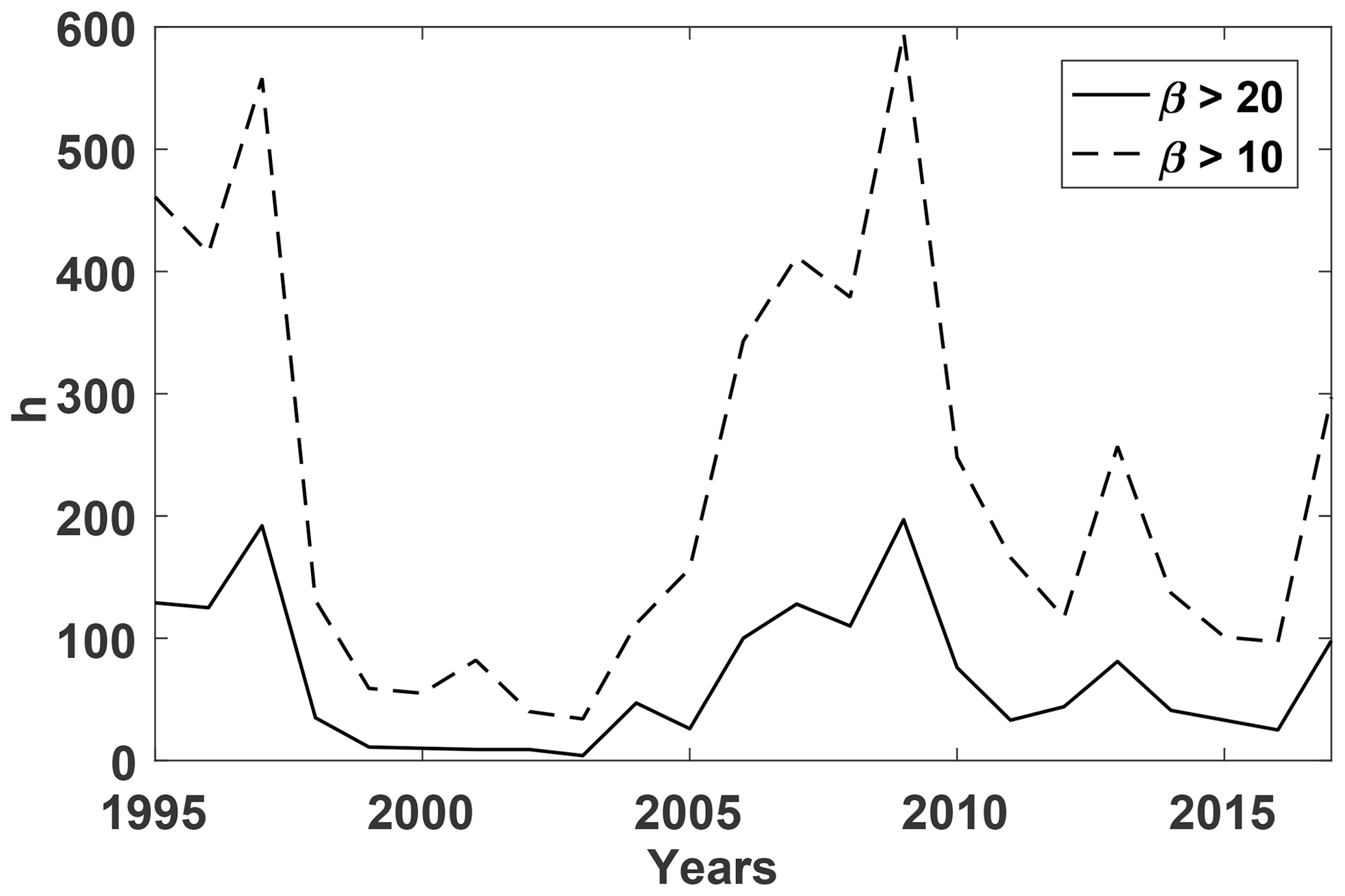
Figure 2 shows the distributions of the magnetic field magnitude, the solar wind speed, density and total static pressure for the full data set of 1 h values during the period from 1995 to 2017 and for the β>10 subset. High β corresponds to slow, cold, and dense solar wind with a low magnetic field (ion temperature not shown here). However, the total static (magnetic plus thermal) pressure distribution is similar (Fig. 2b). Thus, the high-β events are mostly depressions of the magnetic field, compensated for (at least on average) by an increase of plasma density. The only notable difference in the distributions for β>20 (Fig. 2a, red line) is the more frequent presence of the magnetic field ∼1 nT, with an average of 1.6 nT, whereas for β>10 the average is ∼2.2 nT.
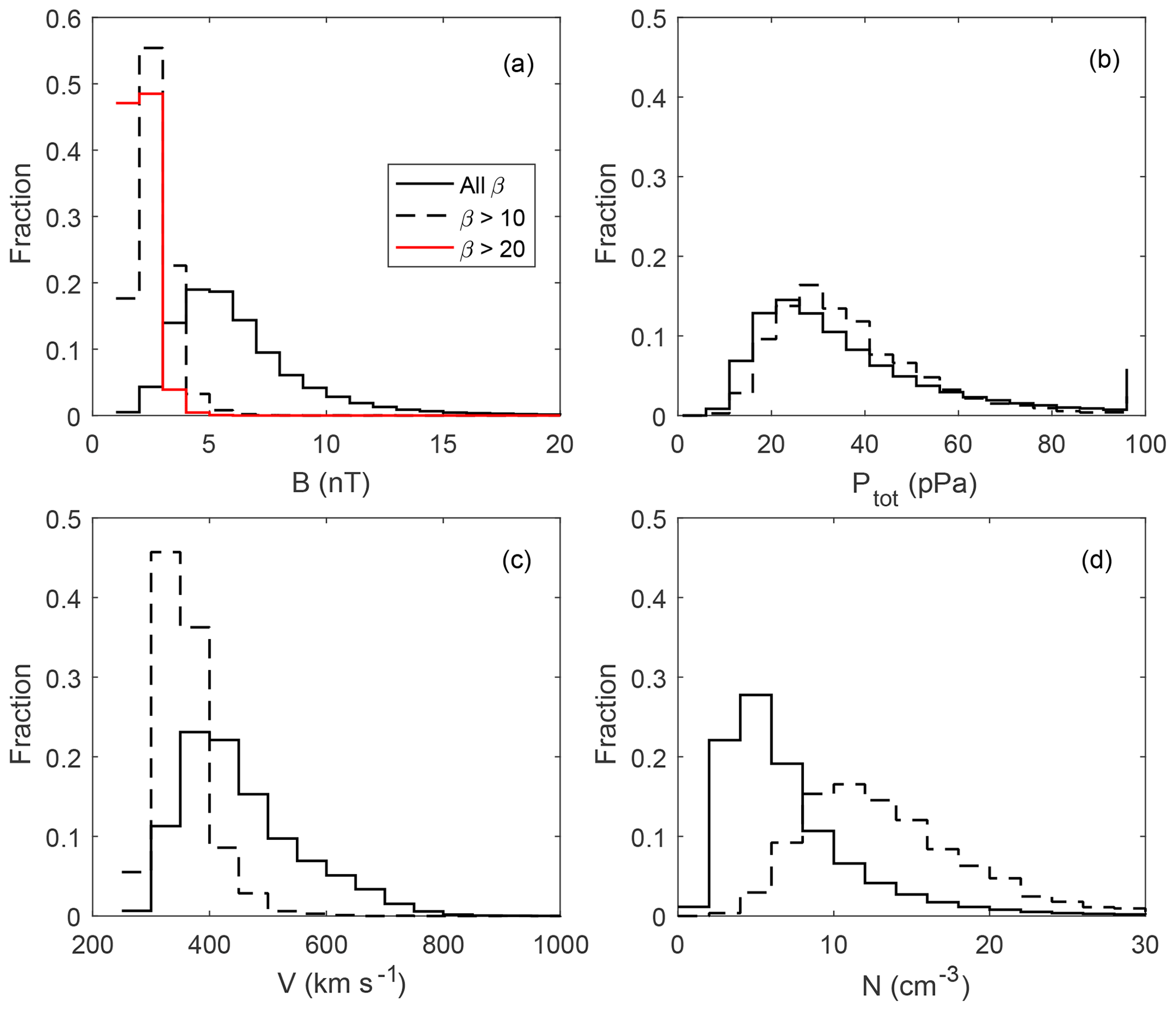
Figure 2Histograms of solar wind and IMF occurrence for 1995–2017 (solid lines) and for the β>10 (dashed lines) subset. (a) Total magnetic field (red line corresponds to β>20); (b) total static pressure; (c) solar wind speed; (d) ion density. The red line β>20 in panel (a) is not given in the other panels, as it is almost identical to the β>10 line.
More than 50 % of events with β>10 have a 1 h duration (one point in the analyzed OMNI variant, not shown here). A sample event is shown in Fig. 3 (here the 1 min OMNI-2 variant is used). There is about a 1 h long decrease in the magnetic field and a density increase, corresponding to β∼20. At an occasional depletion of the magnetic field below 2 nT, β jumps to about 40–80 for few minutes. As the formation of high-β conditions mostly depends on subtle variations in the magnetic field magnitude of around 1–2 nT (note, that β has a square dependence on magnetic field), it should be quite sensitive to the spatial inhomogeneity of the solar wind and IMF, and, in particular, to differences between those detected at L1 (in the OMNI data set) and actually hitting Earth. Figure 4 shows the comparison of the β calculation for the Wind and ACE 1 h data (only for times when Wind data were used in OMNI). The scatter is indeed large. For this OMNI-2 subset there were 618 1 h points with β>10 either in Wind or ACE data. Only 196 of these points had a difference of β at two spacecraft of less than 30 %, while more than half of the events (318) had a difference between the spacecraft of more than 50 %.
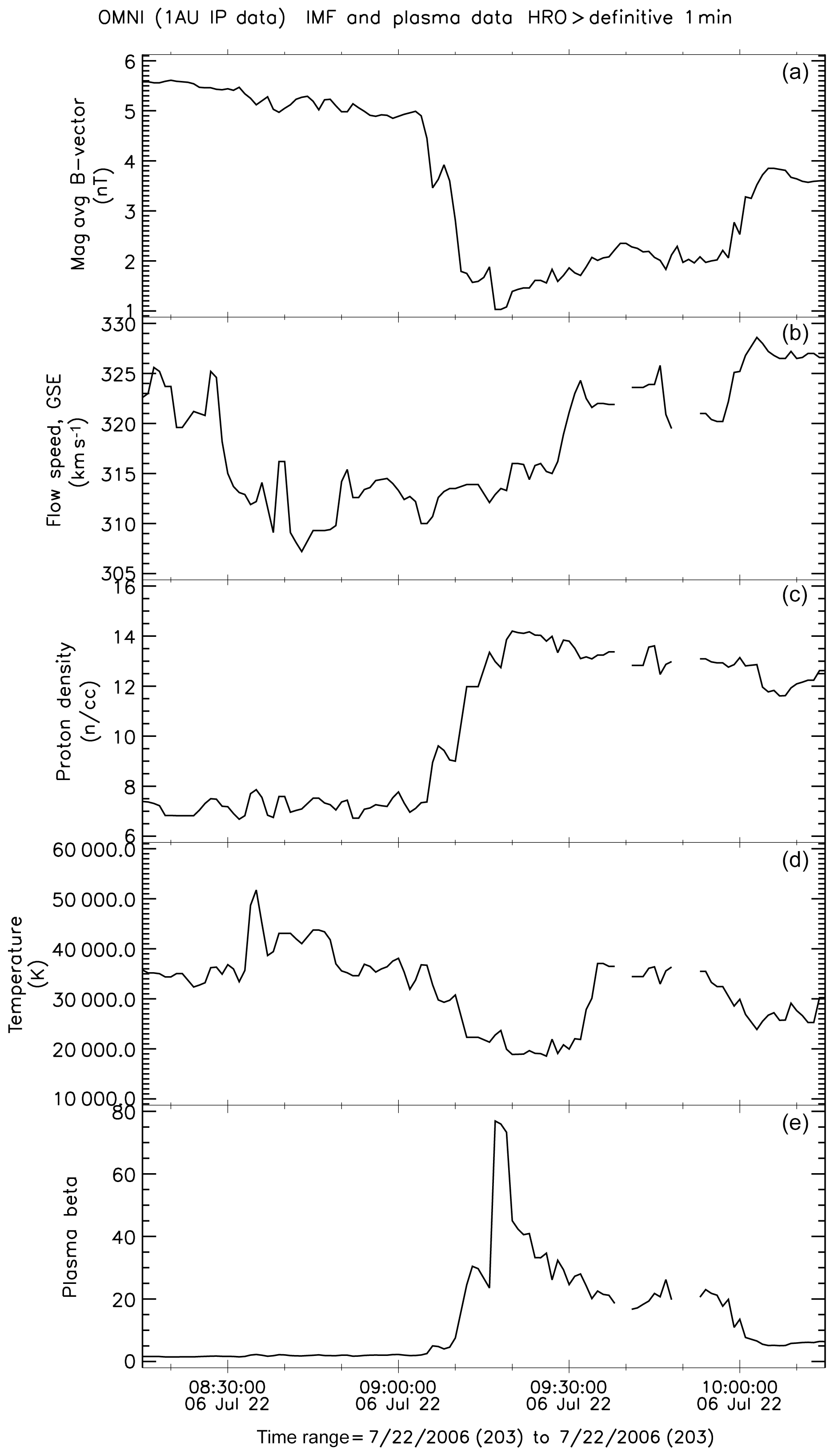
Figure 3Example of the high-β interval. (a) Magnetic field magnitude; (b) solar wind speed; (c) proton density; (d) proton temperature; (e) plasma β. The 1 min OMNI data set was used.
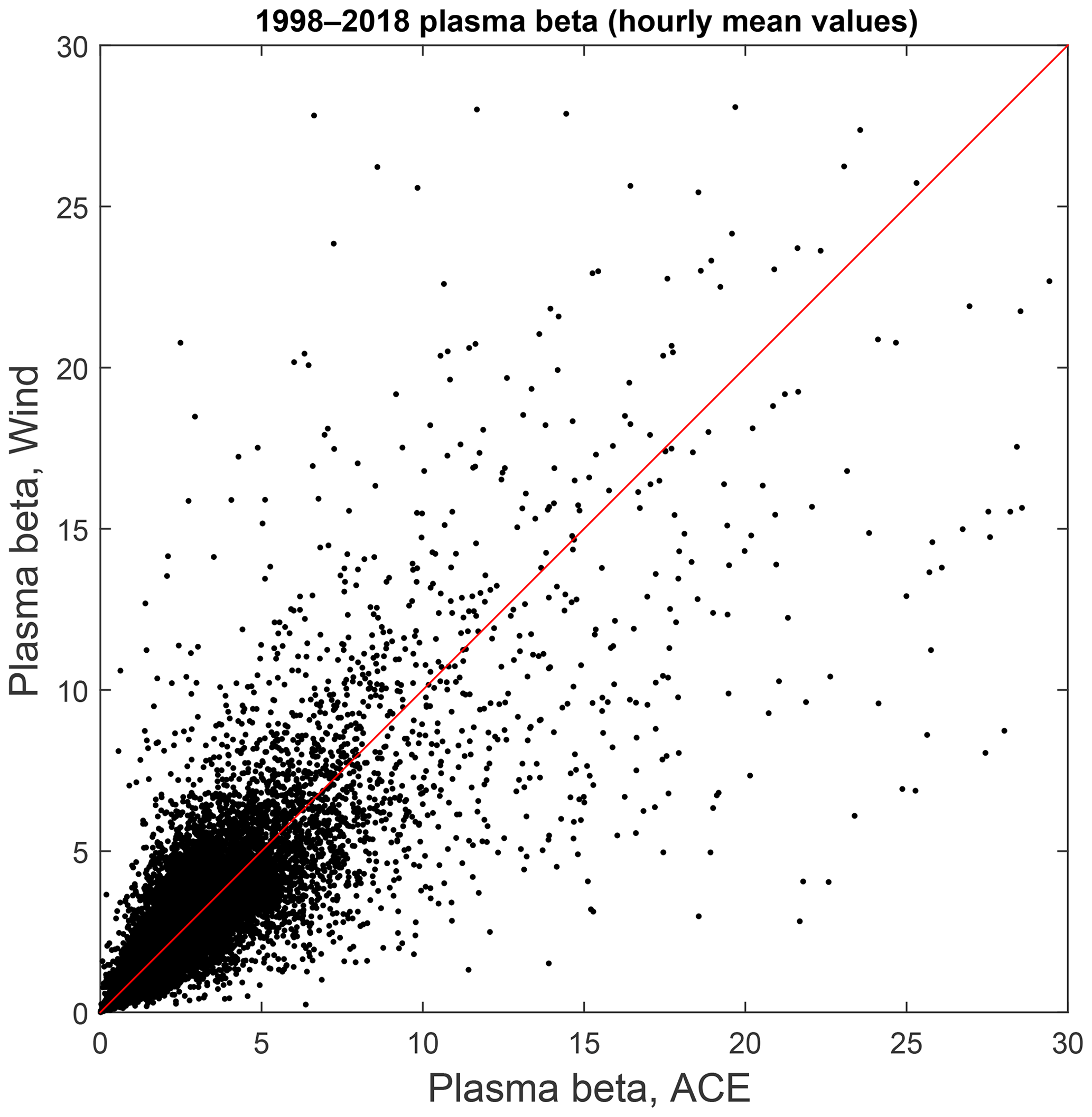
Figure 4Comparison of “Wind” and ACE β using 1 h data. See text for details. The red line is the bisector.
We formulate several conclusions important for our specific shock analysis.
-
Solar wind intervals with high β (β = 10–20) are rare, but not extremely rare, and occur mostly during solar minimum. Thus, some spacecraft (or project phases with a specific orbit or spacecraft separation) may almost completely miss such events.
-
The duration of intervals of interest is relatively short; thus, the selection of shocks with stable upstream conditions may not always be possible.
-
The very low interplanetary magnetic field necessary for high-β events is subject to strong (in relative terms) intrinsic spatial and temporal variability; thus, the actual β conditions and the IMF vector always need to be rechecked using local measurements. This issue is further illustrated by the event selection results below and is elaborated on in Sect. 4.
As high-β shocks are rare, it is unreasonable to search for them by rechecking every registered event. It is more practical to first identify the intervals with the suitable solar wind conditions. A semiautomated algorithm was used to assemble initial statistics regarding shock candidates. For each 1 h point in OMNI with β>10, we check for possible spacecraft located within 5 RE of the model bow shock (Farris et al., 1991). We scanned 1995–2017 observations by all available spacecraft (Geotail, Interball, THEMIS, and Cluster). For this initial selection we use orbital data and spin-averaged magnetic field data from CDAWeb archive.
When a spacecraft is found to be in the right place, the plots of solar wind, IMF, local magnetic field, and plasma parameters are analyzed visually in the 5 h window around the selected hour. These broad temporal and spatial spans are used to ensure that all possible crossings of a moving bow shock are captured for future analysis. Only events with clear shock traversals (jumps in magnetic field and ion density) are accepted. Such manual selection has a definite bias toward quasi-perpendicular and oblique shocks (which usually have a step-like appearance), but this is considered acceptable for this particular study. Most of the initially selected intervals actually did not contain shock crossings.
The shock crossings discovered are checked using the 1 min OMNI data. Plasma β is often below 10, either because the registered shocks are just outside of the initially selected hours, or because β varied on a timescale smaller than an hour. As a change in β is usually accompanied by a solar wind density change, there is also a dynamic pressure change. The latter drives large-scale shock motion and the probability of shock registration by a spacecraft increases. In fact, many shock crossings are registered at a boundary of β change; such events are also discarded, as it is impossible to attribute them to stable upstream plasma conditions.
This preliminary list contains about 100 crossings with an average β of about 20 (taken as the 1 min OMNI value at the moment of shock front crossing). A total of 11 events occurred with very high β>40. The choice of the initial threshold of β>10 (for 1 h points) was finally justified at this stage, as a variant with an initial threshold of β>20 resulted in an almost empty list. However, all of these events still need more detailed confirmation, in particular, regarding the local high β, stable enough crossing velocity, plasma data availability etc.
For the specific multipoint analysis in this investigation, we selected 22 verified Cluster project shock crossings with relatively small spacecraft separation. The full list is given in Table S1 in the Supplement. For the detailed analysis we used a full-resolution Cluster FGM magnetic field (here with the sampling ∼20 Hz) (Balogh et al., 2001) and HIA/CODIF ion data (sampling once every 4–12 s, depending on a parameter) (Rème et al., 2001) from the Cluster Science Archive. As HIA/CODIF data may be not fully reliable with respect to providing ion/proton density (and temperature) in solar wind, we additionally use WHISPER instrument electron density data (Décréau et al., 2001).
One event is from 2003, with a Cluster tetrahedron size of about 300 km, whereas the others are for the later years from 2008 to 2016, when separation between only a pair of Cluster spacecraft C3 and C4 was controlled (30–150 km for our events). This uneven annual distribution is a consequence of the solar cycle dependence (Fig. 1). Events are grouped within a span of 7 non-consecutive days. Specifically, five crossings are registered within 1 h on 18 December 2011, four crossings are registered within 2 h on 3 January 2008, eight crossings are registered within 2 h on 4 January 2008, and two crossings are registered within 1 h on 16 February 2012. However, not all of these adjacent crossings are similar. Three characteristic examples are presented below.
3.1 Event 1
The first example is registered on 18 December 2011 (14:36–14:40 UT) by Cluster C3 and C4 with a separation of 36 km. The spacecraft orbit is almost parallel to the model shock (Fig. 5). Figure 6 contains an overview of the magnetic field and plasma parameters. The solar wind speed is low ∼260 km s−1, and the IMF magnitude is 2.5 nT (all characteristics are given in Table S1). The Alfvén Mach number is ≈18, the magnetosonic Mach number is ≈5, and β (according to 1 min OMNI) is 10.8.
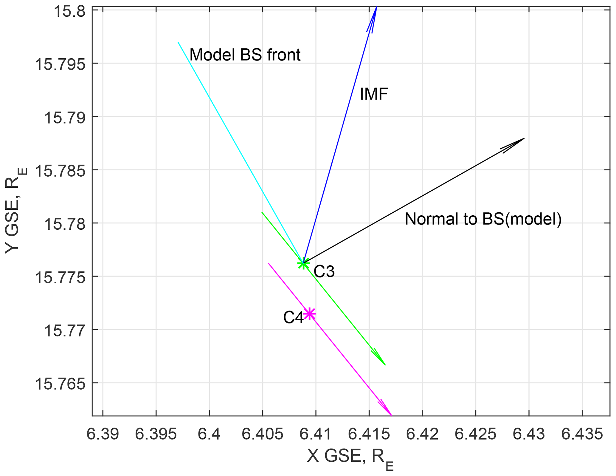
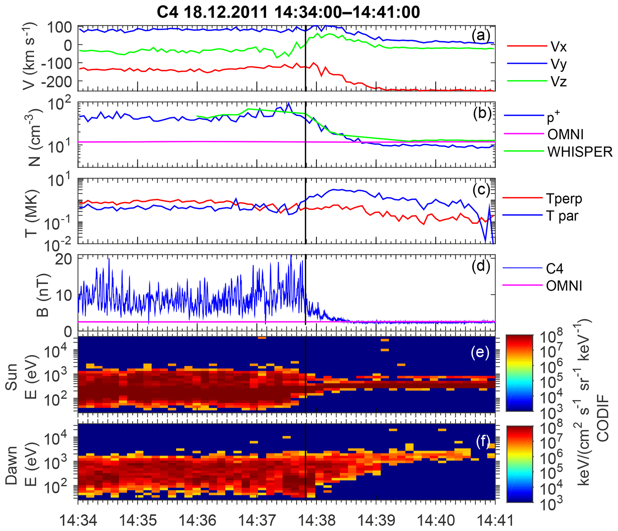
Figure 6Overview of the C4 magnetic and plasma (CODIF) measurements for the event on 18 December 2011. (a) Proton velocity; (b) proton density, OMNI solar wind density, and WHISPER electron density; (c) proton parallel and perpendicular temperature; (d) magnetic field magnitude and OMNI IMF magnitude; (e) proton spectrogram for the sunward-looking sector; (f) proton spectrogram for the dawnward-looking sector.
The ion (proton) density in the solar wind according to Cluster is lower, than that in OMNI. However, the WHISPER electron density is almost the same. The proton perpendicular temperature grows as expected in the downstream direction, whereas the parallel temperature peaks just upstream of the shock front. We attribute this peak to upstream-moving field-aligned protons. The presence of two populations with strongly different flow velocity results in the false temperature increase. Thus, using local ion data to calculate local β would be unreliable. We confirm β using only the local magnetic field, as it is the most variable parameter (in comparison with the plasma density). The solar wind magnetic field measured locally by Cluster is the same as OMNI data (compare the two lines in Fig. 6d). The OMNI IMF vector direction is ∼10∘ different, with the local upstream field taken at 14:40–14:41 UT (not shown here).
The model shock normal angle θBn with respect to OMNI (local) IMF is 46∘ (54∘) (using Farris et al., 1991 model). The coplanarity calculation for the shock normal results in a θBn that is equal to 42∘. Downstream and upstream intervals were taken as 14:36–14:37 and 14:40–14:41 UT, respectively. Thus this is quasi-perpendicular or oblique supercritical bow shock with reliably determined geometry. Such crossings for more standard β are well studied (Scudder et al., 1986; Krasnoselskikh et al., 2013; Lefebvre et al., 2009). The compression ratios for the magnetic field and plasma density are 3.55 and 3.65, respectively.
The shock transition lasts for about 200 s (14:37:00–14:40:30 UT) from the first signs of the upstream high-energy ions, which can be observed on the spectrogram in Fig. 6f up to the stable downstream conditions.
The increase in the magnetic field magnitude and ion density (shock ramp in a quasi-perpendicular case) is smeared over half a minute (14:37:45–14:38:20 UT). The nominal shock front transition is somewhat arbitrarily placed at 14:37:45 UT (marked by vertical line) at a first extended peak of the magnetic field. The magnetic field increase has no regular or step-like form, and the magnetic magnitude immediately downstream is often as low as 5 nT. Thus, it is impossible to determine the shock speed by comparing C3 and C4 measurements.
However, Cluster 2, about 6000 km away from the C3 and C4 pair, crossed the shock 2 min later (the exact values are 6231 km and 124 s between C3 and C2, but this is not shown here). The separation of C3 and C2 along the model normal is 1032 km, and the spacecraft pair is elongated along the shock front. The shock speed along the normal is 8.3 km s−1 outbound. This calculation is not very reliable for two reasons. (1) The spacecraft are mostly separated along the front by about 6000 km, and the shock motion may be different in two so different points. (2) The subsequent crossing in the reverse direction occurred less than 10 min later; thus, the shock speed might substantially change on a scale of 2 min (separation between C3 and C2). Nevertheless, one can estimate the spatial scale of the ramp. A duration of 35 s corresponds to 290 km. The convective gyroradius of a solar wind proton in IMF is ∼1200 km, in the downstream magnetic field it is 380 km, and the ion inertial length in solar wind is ∼66 km (in these estimates we neglected small shock speed).
In Fig. 7, we highlight the interval with the strongest low-frequency magnetic variations. Frequency spectra are shown in Fig. 8. The magnetic profile is dominated by a variation with frequency of around 0.3 Hz and an amplitude up to 20 nT, which is more pronounced in By. An interval of 14:37:27–14:37:47 UT is taken to estimate the wavelength. As the variation has a clear dominant frequency, it is more convenient to perform time-domain multipoint analysis.
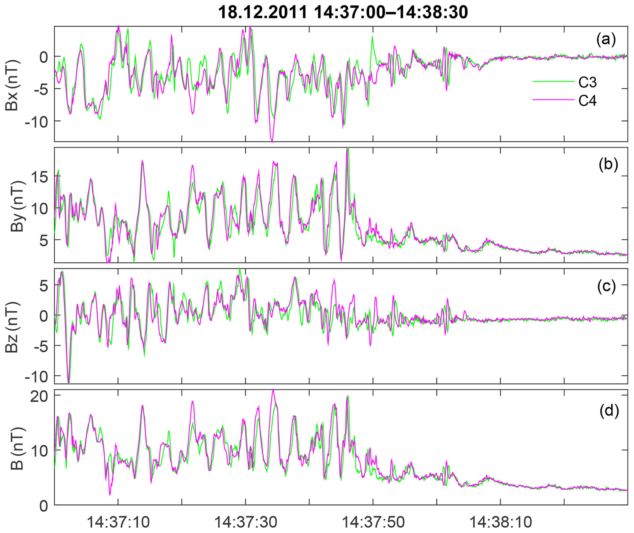
Figure 7Full-resolution magnetic waveform for the shock on 18 December 2011. Panels (a)–(d) show the components and the total value of the magnetic field.
Parameters of magnetic variations, filtered in a frequency range from 0.1 to 0.77 Hz are presented in Table 1. The vector of maximum variance is almost along the local magnetic field (By component dominates), whereas the vector of of minimum variance is along Z. Ratios of eigenvalues are and , and one may assume elliptic polarization. The time shift between magnetic measurements along the maximum variance component, determined with the correlation analysis, is 0.13 s. This value is rather reliably calculated, as it is 2–3 times larger than the sampling interval. This shift is also persistently visible in the relevant interval in Fig. 7a and b. The spacecraft separation along the minimum variance direction is 10 km, and the resulting wavelength estimate is ∼250 km.
Table 1Wave analysis data for the shock on 18 December 2011, 14:37:27–14:37:47.
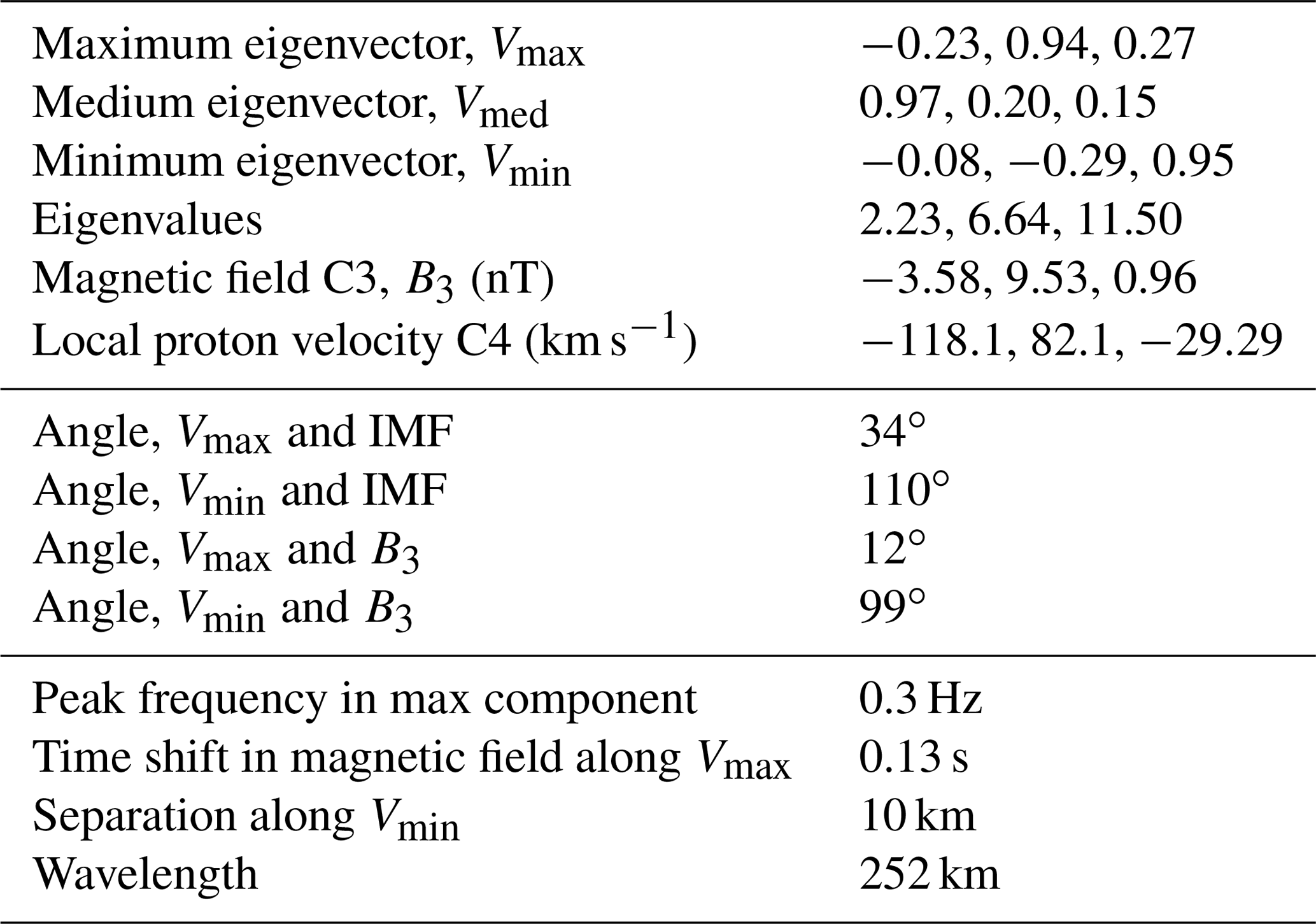
However, the hodograph of the magnetic field rotation (Fig. 9) shows that the polarization might actually be linear with the maximum variance direction changing every several periods (two variants are shown by red lines). In a case such as this, the propagation direction cannot be defined with the variance analysis. For compressive low-frequency MHD waves the propagation direction can be determined with the coplanarity approach (Hubert et al., 1998). Namely, the maximum variance direction, the magnetic field direction, and the wave vector should be in the same plane. In this case, the angle between the maximum variance direction and the local magnetic field is rather small (only 12∘) and a coplanarity calculation would be unreliable.
We also estimate the span of principally possible wavelengths. The maximal one is ∼900 km, which was obtained by taking full spacecraft separation (36 km). Both estimates (250 and 900 km) are approximately equal to or larger than the local ion gyroradius (330 km, introduced above). The Doppler shift is 0.04–0.58 Hz, depending on the wavelength and the assumed local proton velocity value (full 146 km s−1 or its projection to the minimum variance eigenvector 41 km s−1).
Finally, we note the oscillations with a higher frequency of about 1 Hz and a smaller amplitude of a couple of nanotesla (nT), which are best observable in the Bz component (Figs. 7c, 8). The eigenvalue ratios (after filtering the frequency range from 0.7 to 10 Hz) are and ; thus, the reliable determination of any wave proper direction is definitely not possible. Oscillations are quite different at two spacecraft, and the multipoint analysis also proved not to be possible.
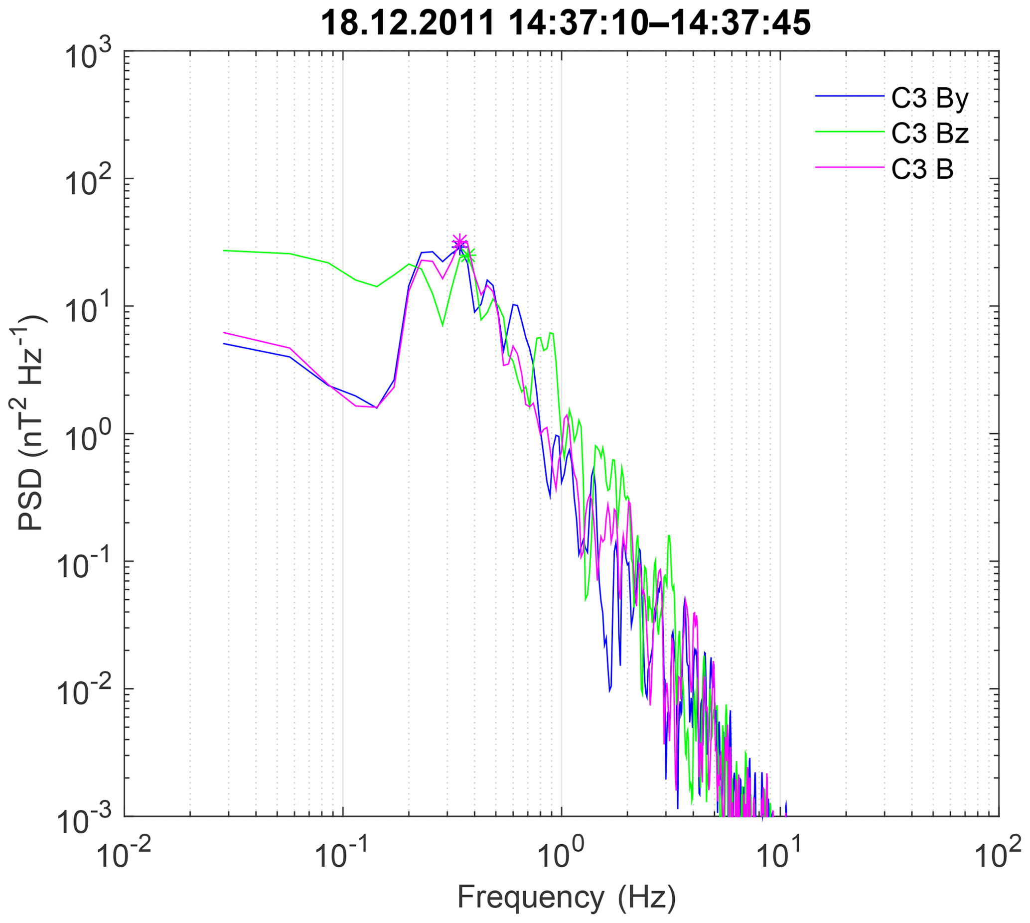
Figure 8C3 frequency spectra for the By and Bz components and the magnetic field magnitude for the shock on 18 December 2011.
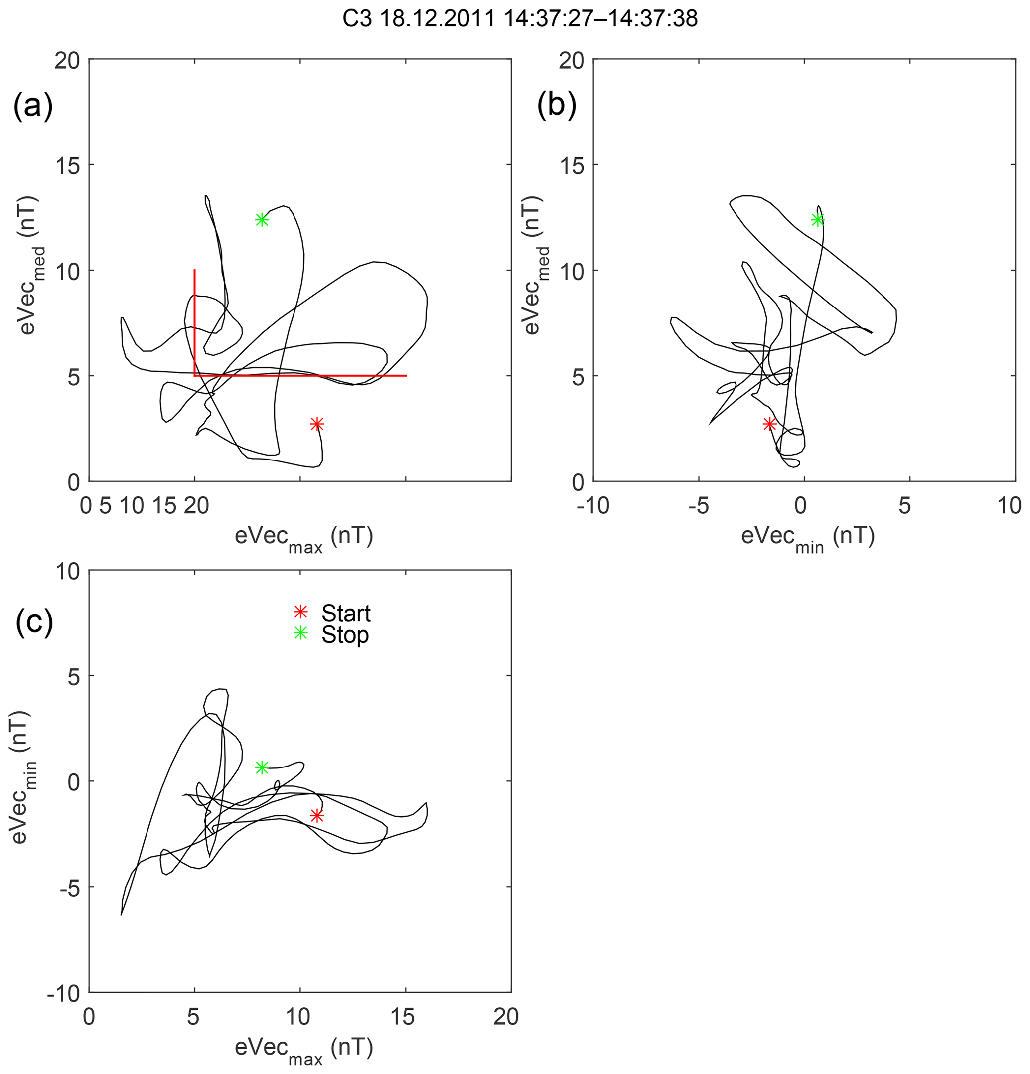
Figure 9Hodographs of the C3 magnetic field in eigenvector coordinates for the shock on 18 December 2011. Two variants of linear polarization are highlighted by red lines in panel (a).
3.2 Event 2
A shock from 4 January 2008 (16:00–16:04 UT) was registered with Cluster C3 and C4 separation of about 40 km. The general event parameters are given in Table S1, and an overview of the plasma and magnetic field parameters are given in Fig. S1 in the Supplement. The detailed wave activity at the front is presented in Fig. 10. Solar wind parameters and general crossing structure are very similar to those for Event 1. The solar wind speed is low ∼315 km s−1, and the IMF magnitude is 2.4 nT. The Alfvén Mach number is ≈23, the magnetosonic Mach number is ≈7, and β (according to 1 min OMNI) is 12.2. The solar wind magnetic field measured locally by Cluster is the same as OMNI data (compare the two lines in Fig. S1d); therefore, the OMNI β value is confirmed. All variants for θBn give ∼40∘.
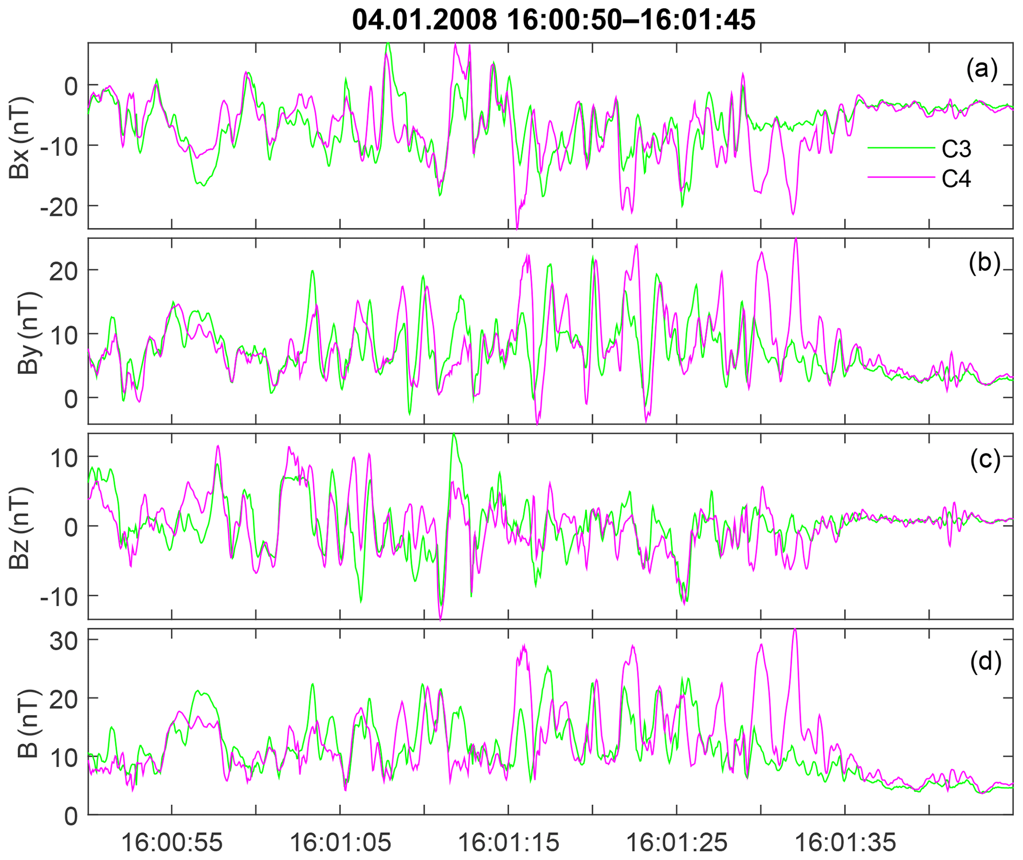
Figure 10Full-resolution magnetic waveform for the shock on 4 January 2008. Panels (a)–(d) show the components and the total value of the magnetic field.
The transition lasts about 2 min (16:00:50–16:02:50 UT) from the first signs of upstream high-energy ions and ion velocity change to the stable downstream conditions (Fig. S1f). The jump in the magnetic field magnitude and ion density is smeared over half a minute from 16:01:30 to 16:02:00 UT, and is wavy rather than step-like; the downstream magnetic magnitude is often as low as 2–5 nT. The nominal shock front transition is somewhat arbitrarily placed at 16:01:35 UT at a first extended peak of the magnetic field.
In general, this ramp transition is a slow ≈30 s long simultaneous increase of the magnetic field and ion density, which is visually similar to Event 1. Characteristic plasma scales for Event 2 are almost equal to the values for Event 1. Compared with the C2 location (not shown here), the spacecraft separation is more than 11 000 km, whereas the separation along the model normal is much smaller (about 100 km). The estimated shock speed is 1.5–2.2 km s−1 (comparing the C3–C2 and C4–C2 pairs), which corresponds to a ramp width of about 50 km. However, this estimate is very unreliable, as it would strongly depend on small variations of the actual normal.
The full-resolution waveform is shown in Fig. 10. Similar to Event 1, there is a dominating oscillation with a frequency of about 0.4–0.5 Hz, as well as lower amplitude waves with a frequency of above 1 Hz (Fig. S2). The specific feature of this event is a strong difference in C3 and C4 variations during the first 20 s downstream of the front (16:01:25–16:01:35 UT), despite relatively small separation. The substantial difference in waveforms also remains further downstream. This is true for all other shocks registered during this day as well (eight crossings within 2 h in Table S1).
Despite these differences, it is possible to perform multipoint separation analysis for the interval from 16:01:15 to 16:01:25 UT, where two waveforms in the By component (Fig. 10b) are more similar and are shifted by a fraction of a period. All wave parameters (filtered in the range from 0.1 to 2 Hz) are shown in Table 2. As in Event 1, the maximum variance eigenvector is almost along Y, and the medium eigenvector is along X. Ratios of eigenvalues are and ; thus, the minimum variance (nominal propagation) direction is well defined. The time shift between the magnetic measurements along the maximum variance component is 0.22 s (determined with correlation analysis), whereas the spacecraft separation along the minimum variance direction is 6.8 km. The resulting wavelength estimate is 61 km for the peak frequency of 0.5 Hz. This value is close to the spacecraft separation distance (about 40 km) and, thus, is generally consistent with the observed substantial difference between magnetic fields at C3 and C4.
Table 2Wave analysis data for the shock on 4 January 2008, 16:01:15–16:01:25.
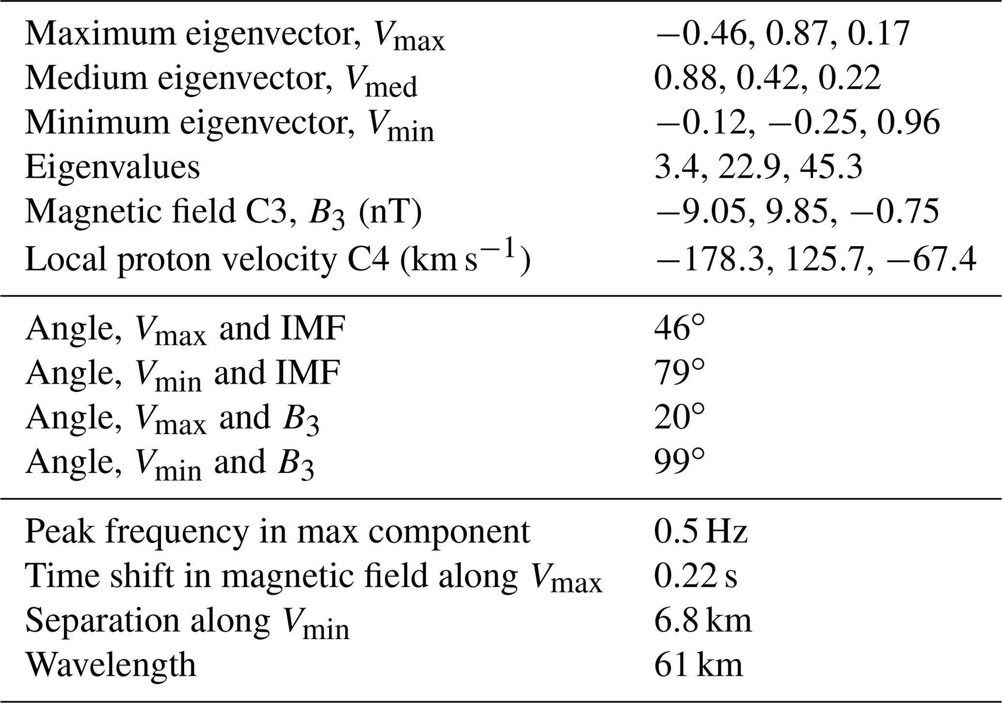
The hodograph of the magnetic field rotation (Fig. 11), however, shows the absence of any stable polarization. It can be interpreted as linear for a couple of periods, and then almost circular for some periods (most clear in Fig. 11a with the maximum and middle variance vectors). The coplanarity approach can again not be used here to confirm the wave-vector direction, as the angle between the maximum variance direction and the local magnetic field is rather small (20∘). The maximum possible wavelength (if the spacecraft separation along the wave vector is maximal 40 km) is ∼400 km.
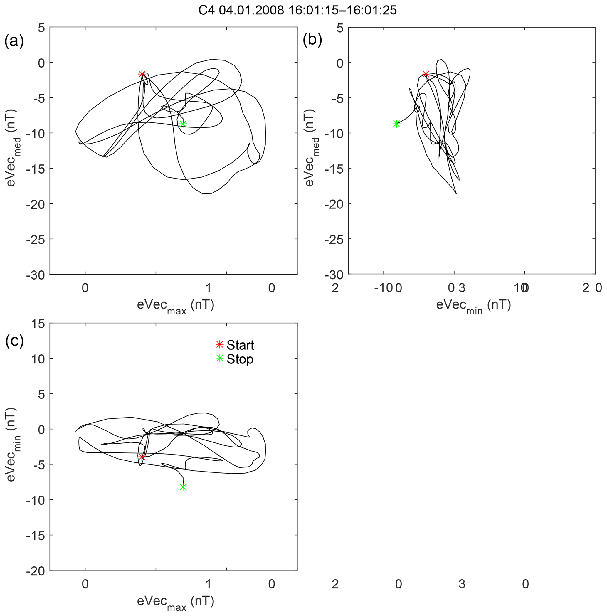
Figure 11Hodographs of the C4 magnetic field in eigenvector coordinates for the shock on 4 January 2008.
3.3 Event 3
One more example is from 3 January 2008 (14:30–14:35 UT) with Cluster separation of ∼100 km (Table S1 and Fig. S3 in the Supplement). OMNI data showed very low IMF (1.1 nT) and β=39. The solar wind speed is low ∼321 km s−1, the Alfvén Mach number is ≈42, and the magnetosonic Mach number is ≈7. The model θBn is 47∘. In Fig. 12 we present the local magnetic field along with OMNI data. Although the local upstream magnitude is approximately equal to that in OMNI (except starting from 14:30 UT closer to the shock), the upstream field direction changes by more than 90∘ and the local model θBn also changes to more perpendicular geometry. The presence of an earlier shock crossing at 14:20 UT may also affect observed upstream conditions. Strong changes of the magnetic field direction on a scale of 1 min are also present downstream of the shock (Fig. 12, right side). Therefore, for this shock, reliable determination of magnetic geometry is impossible.
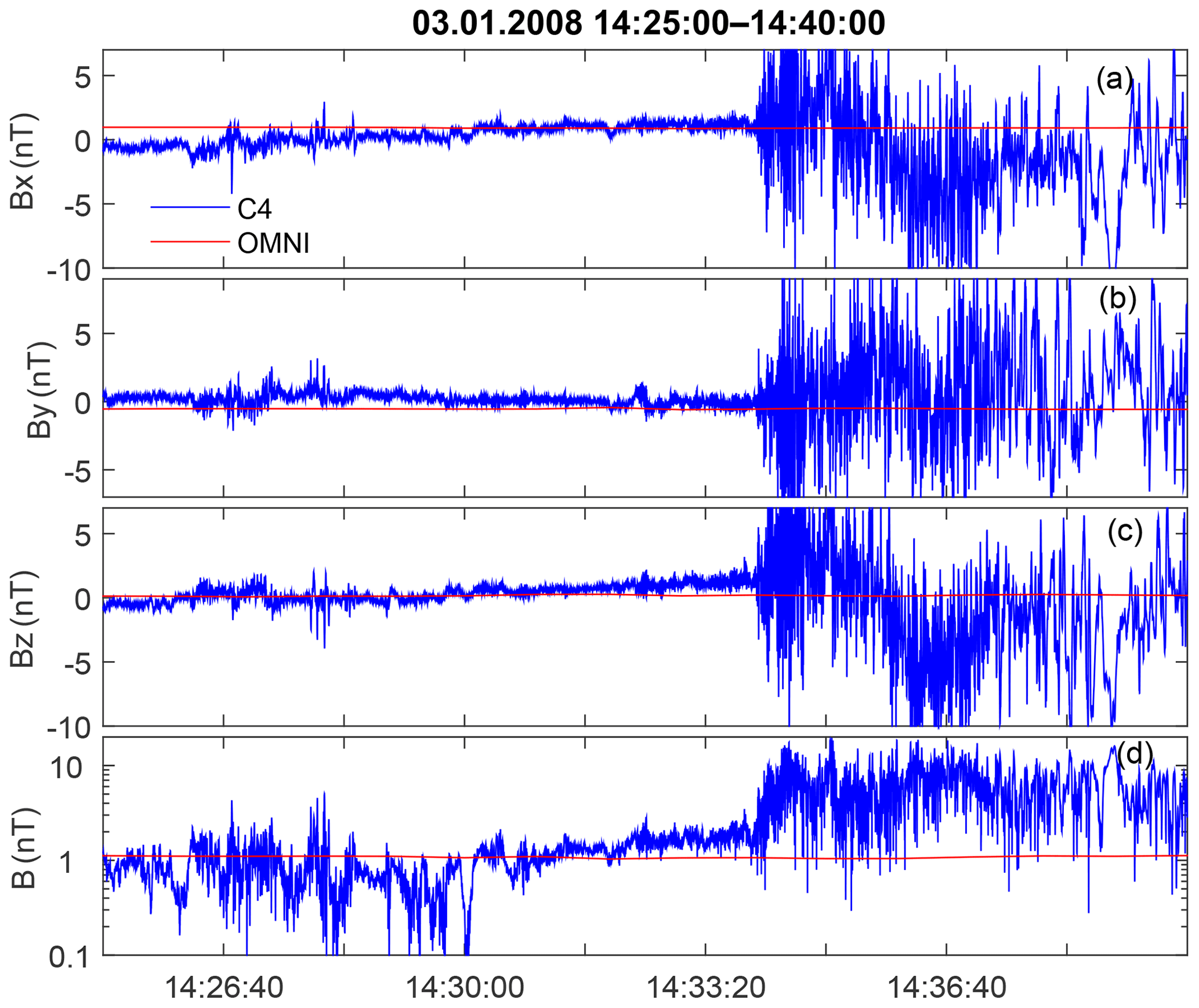
Figure 12The local upstream and OMNI magnetic field for the shock on 3 January 2008. Panels (a)–(d) show the components and the total value of the magnetic field.
Figure S3 contains an overview of the magnetic field and plasma parameters. The transition lasts about 2.5 min, from 14:32:00 to 14:34:30 UT, from the first sign of ion velocity change, upstream high-energy ions, and growth of parallel ion temperature (Fig. S3e, f) to the stable downstream conditions. The jump in magnetic field magnitude is smeared over about half a minute, from 14:34:00 to 14:34:30 UT, is wavy, and the magnetic magnitude downstream is often as small as 1–2 nT. The nominal shock front transition is somewhat arbitrarily placed at 14:34:10 UT (marked by a vertical line in Fig. S3). Some increase in the variation amplitudes around 14:34:10 UT can be interpreted as a localized intensification or as a result of shock bounce motion. The ion density increase at the ramp does not coincide with the magnetic field increase and is longer lasting.
Similar to Event 1, one can estimate shock speed along the normal, comparing with C2 (not shown here). The spacecraft separation is 5700–5800 km, whereas the separation along the model normal is 1400 km. The estimated shock speed is 11 km s−1, which corresponds to a ramp width of about 330 km. The convective gyroradius of solar wind protons in IMF is about 2400 km, in the downstream magnetic field it is 540 km, and the proton inertial length in solar wind is 83 km.
A detailed view of the magnetic variations is given in Fig. 13. Only relatively high-frequency oscillations of about 2 Hz are present (frequency spectra are shown in Fig. S4). There are no wave packets with the stable phase. For example, at 14:34:10–14:34:14 UT, X and Z components are in anticorrelation for C3 and C4, while in close proximity, at 14:34:08–14:34:10 UT, these components are in phase. Therefore, a reliable multipoint analysis for this event is impossible. A magnetic field hodograph plot for 14:34:10–14:34:14 UT is given in Fig. 14. It confirms unstable (but consistent with the changing linear) polarization. Assuming that C3 and C4 variations are mostly in antiphase (half a period between the spacecraft), the maximal wavelength is estimated to be ∼200 km.
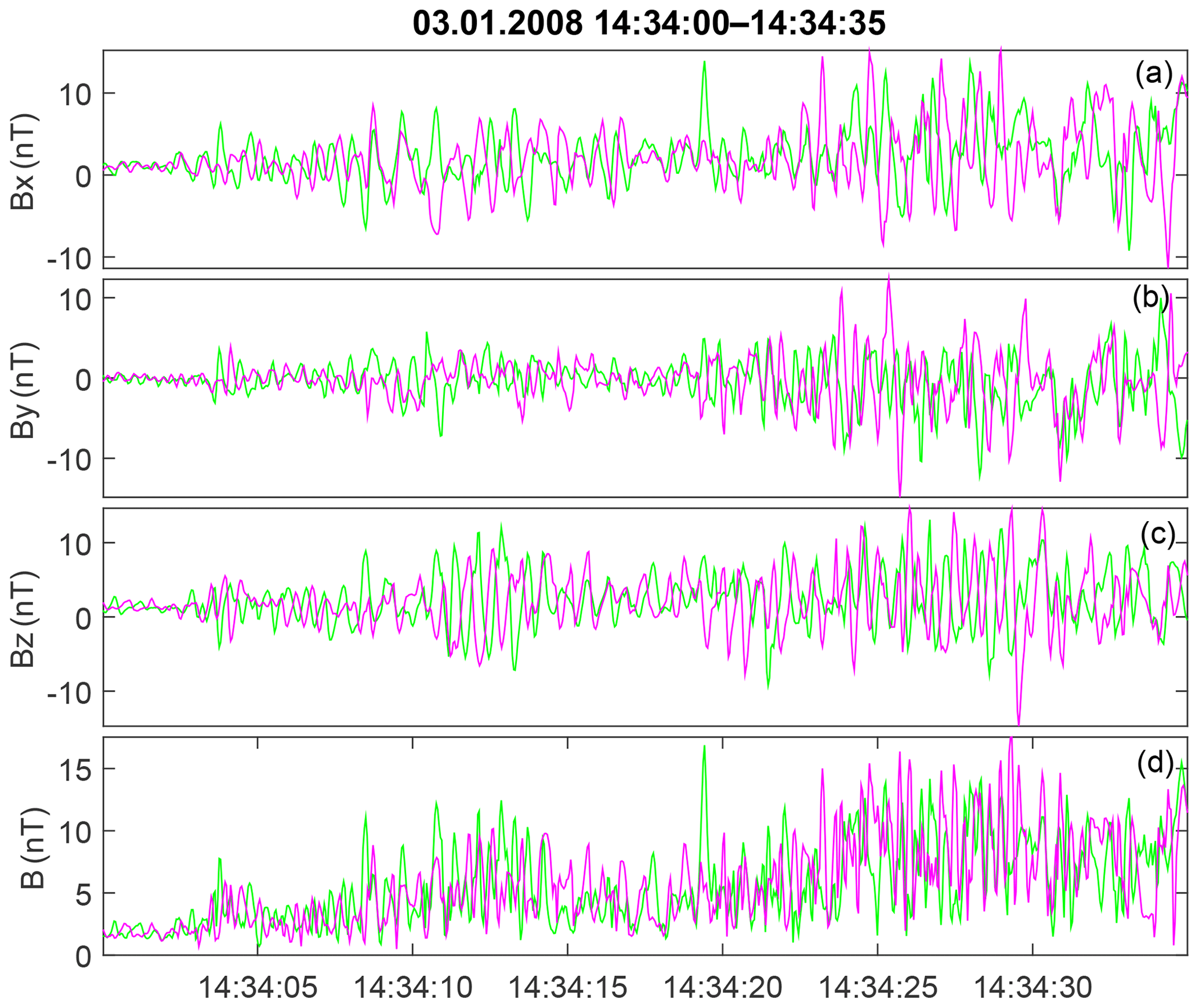
Figure 13Full-resolution magnetic waveform for the shock on 3 January 2008. Panels (a)–(d) show the components and the total value of the magnetic field. The color-coding is the same as in Figs. 7 and 10.
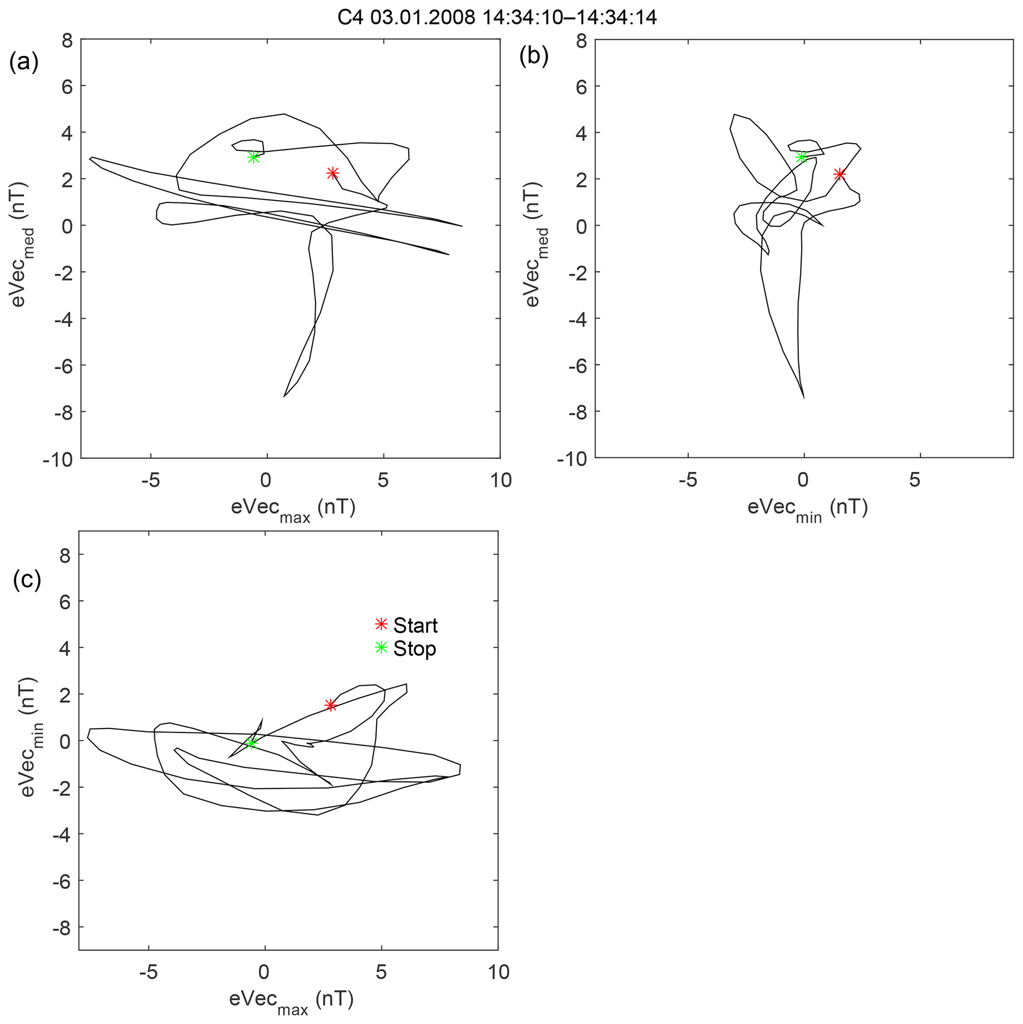
Figure 14Hodographs of the C4 magnetic field in eigenvector coordinates for the shock on 3 January 2008 for 14:34:10–14:34:14.
3.4 Observation summary and statistics
Our statistics include 22 oblique and quasi-perpendicular shocks. The three examples above illustrate the typical shock properties well. The minimum θBn is 37∘, and the two largest ones are 62 and 83∘. Values of β range from 39 to 7.5. All cases are supercritical shocks with magnetosonic Mach numbers more than 5.5. The Alfvén Mach numbers are large due to large β values. All shocks exhibit a clear several-minute-long transition zone between pristine solar wind ion flow and magnetosheath. The somewhat smeared main magnetic field and density increase lasts roughly several tens of seconds or several hundred kilometers. This magnetic profile is typical for all of our shocks irrespective of the θBn angle.
On a smaller timescale of seconds, the magnetic profile is dominated by magnetic variations much larger than the background field, which gradually grow across the magnetic ramp in the downstream direction. As a result, the exact location of the “main” magnetic jump cannot be defined.
The three examples show characteristics of the dominating magnetic variations, which are typical for all of the events considered. The detailed multipoint variation analysis allowed us to obtain the following new information. In most of the shocks (and in events 1 and 2) the variations exhibit the well-defined frequency peak of ∼0.2–0.5 Hz. The phase of these variations is irregular, with no clear persistent polarization. It can also be interpreted as a linear polarization with the frequently changing the main direction. However, as the amplitude of the variations is larger than the background field, the main axis of linear polarization is almost always along the field vector. Such polarization does not allow us to reliably determine the wave propagation direction and the wavelength. We only get estimates in the range of several tens to several hundreds of kilometers.
Two shock events (31 December 2003 and our Event 3 on 3 January 2008 14:32 UT) have dominating ∼2 Hz variations, which are visually notable due to the more harmonic waveform, but also have an unstable phase. The spatial scale of these variations is smaller than the spacecraft separation, so that it proved to be impossible to determine with multipoint data. These two shocks are similar to the other events in terms of their other general parameters. Moreover, one of them (Event 3 above) is registered just 10 min after a crossing, which exhibited the first type of variations.
4.1 The reliability of solar wind input
High-β solar wind is relatively rare at the Earth orbit. In our study we accepted a somewhat ad-hoc threshold of high β equal to 10. Such interplanetary conditions tend to occur during solar minima, and are created by slow, cold, dense solar wind with low IMF (1–2 nT). However, is not always easy to confirm that the observed shock crossing actually occurred in a high-β solar wind interval, identified in OMNI. The first set of problems is related to the association of particular crossings with stable high β. These problems are relatively straightforward to identify in data. A more substantial problem is related to the inherent solar wind and IMF variability. We measure solar wind at the L1 halo orbit, 1.5 million kilometers from Earth and with a halo radius of no less than 200 000 km (for ACE spacecraft). A substantial part of modern OMNI data are taken from the Wind spacecraft, which is currently on a much wider halo orbit (300–400 000 km) (Podladchikova et al., 2018). The solar wind and IMF structures at L1 are not necessarily the same as those that actually affect the magnetosphere. The most questionable is the spatial persistence of relatively small changes of IMF from 2 to 1 nT, which are required for the creation of very high-β intervals.
Although the specific analysis of the spatial scales of high-β areas in solar wind was not performed, available reports indicate significant potential problems. The ISEE data study suggested that during periods of medium to low magnetic field variance, magnetic features with scales of about 20 RE perpendicular to IMF may occur (Crooker et al., 1982). Comparison of L1 Wind and near-Earth Interball data for 1996–1999 (Petrukovich et al., 2001) has shown that IMF structures, associated with geomagnetic storms (with an IMF Bz GSM threshold below −10 nT over 3 h), are practically the same at the L1 and the near-Earth orbits. However, about 20 %–80 % of the smaller everyday IMF variations, which cause substorms (several nanotesla in magnitude on a 1 h scale), differ by more than 25 %.
Thus, very high β values in OMNI are not readily applicable for a shock study. It is not always possible to check solar wind β immediately before a shock crossing. A spacecraft needs to probe pristine solar wind and then rapidly cross the shock, or there should be an additional near-Earth solar wind monitor. The magnetic field can be reliably measured using a magnetometer (still assuming an offset uncertainty of about 0.1 nT). The comparison of ion density and temperature measurements is more problematic. Assumptions regarding the constant helium content and constant electron temperature, used in OMNI β calculations, may also result in some errors. For example, a factor of 2 change in electron temperature will result in an approximate 30 % change in β. A factor of 2 variation in the He++ content will result in an approximate 10 % variation in β. Of course, additional (relative to those found in the OMNI set) high-β intervals may actually form near the bow shock, as a side product of such variability.
4.2 General shock properties
The relatively compact large-scale structure of the observed shock transitions (about a couple of minutes) is similar to that reported for oblique and quasi perpendicular shocks. It is distinctly different from the structure of quasi-parallel shocks, which are extended up to several Earth radii (Burgess et al., 2005).
The apparent increased width of the magnetic jump in our cases (∼30 s) might be related to the larger ion gyroradius in the high-β plasma and the relatively slow shock motion (only about 10 km s−1). In fact, for Event 1 and Event 3, where it was possible to estimate the spatial scale, the ramp length (divided by 2) was about 0.5 of the convective proton gyroradius in the downstream field and about 2–3 time larger than the ion inertial length in the solar wind, which is consistent with the statistics of Bale et al. (2003).
Magnetic variations during this ramp-like increase have an amplitude comparable with or larger than the background magnetic field, so that there is no “stable” magnetic structure on timescales of seconds. In comparison, for a supercritical quasi-perpendicular low-β shock, one usually defines (starting from the upstream) the prolonged interval of somewhat enhanced density and magnetic field (shock foot – lasting tens of seconds) and the sharp main increase (ramp – lasting seconds). The ramp is often used to determine the shock motion with multipoint measurements, but in our case it is impossible.
A more detailed phenomenological description of this shock transition requires the analysis of ion kinetics, which will be performed elsewhere. The possible dependence of shock spatial scale on β is an interesting aspect and should be addressed in future studies on larger statistics.
4.3 Magnetic variation properties
Observations of the high-amplitude magnetic variations and the absence of a sharp ramp profile in high-β events are similar to those presented earlier by Formisano et al. (1975) and Farris et al. (1992) (as far as it can be discerned by visual examination of figures). In this investigation we improved our knowledge by analyzing spectral and polarization properties of these variations.
With two Cluster spacecraft separated by several tens of kilometers, it was possible to estimate the spatial scale of these dominating variations. Three typical variants were found. In some events (Event 1) variations had a rather irregular form, a typical frequency of about 0.5 Hz, and were very similar on the two spacecraft, suggesting a scale of some hundred kilometers. The second spatial scale variant is illustrated by Event 2. It includes variations visually similar to those in Event 1, but with a mix of scales of the order of 100 km, which can be captured with our spacecraft separation, and of the order of tens of kilometers. As a result, the waveforms are rather different, but common features can sometimes be traced. Finally, the third variant (Event 3) contains more harmonic waves with higher frequencies of around 1–2 Hz and the quantitatively unresolved dominating spatial scale of 200 km at most.
The observed variations are very different from those in low-β supercritical events (e.g., Krasnoselskikh et al., 2013), where clear whistler wave packets with elliptic polarization dominate. Observed polarization is also not consistent with the Alfvén mode, which was suggested earlier for high-β shock (Coroniti, 1970; Kennel and Sagdeev, 1967).
The wavelength can be determined independently from the propagation direction with only four measuring points. Alternatively one can fix the propagation direction with the minimum variance analysis in the case of elliptic polarization or with the coplanarity supposition. Unfortunately, in our cases it proved impossible to determine the wave-vector direction reliably using either method, as we have linearly polarized waves with a maximum variance direction along the main magnetic field. Note, that such a configuration is inevitable for a variation much larger than the background field.
Linear polarization with a very high amplitude, substantially changing the total magnetic field, suggests strong nonlinearity and a compressive nature. The absence of any several-period-long wave packets with the stable phase also suggests strong spatial localization.
The dominating wave mode downstream of the shock front was also addressed in a number of other investigations; however, cases of really high β>10 were not specifically addressed. Hubert et al. (1989) identified the mirror waves, comparing magnetic field with density, provided by the fast electron measurements of the ISEE project. Balikhin et al. (1997) identified the intermediate mode with two-point AMPTE data analysis. Lacombe et al. (1992) suggested the mirror mode with linear polarization for higher-β shocks, and successfully used the coplanarity assumption to define the wave-vector direction. Czaykowska et al. (2001) showed the compressive mode as well as the left-hand polarized mode in shocks with β>1. Therefore, almost the full variety of possible wave mode variants have been identified.
A definite plasma mode analysis critically depends on the reliable determination of the wave propagation (wave-vector) direction, which proved to be impossible in our cases. Also, it should be noted that all studies referenced above used several-minute data intervals, which were often several minutes away from the shock transition, with the natural motivation to access the long sets of uniform variations. In the most cases, the analyzed frequencies were below 0.1 Hz. This approach is different from ours, in which we addressed relatively short intervals of the most powerful oscillations.
An alternative wave mode candidate, frequently suggested for high-β plasma, is the Weibel instability, which is fundamentally similar to the drift mirror mode. With no seed magnetic field, the Weibel mode only has imaginary frequency, in which magnetic field variations are growing faster than they propagate. For a finite magnetic field, Pokhotelov and Balikhin (2012) suggested that the Weibel mode grows as a mix of two opposite circular polarizations and attains some small real part of frequency. Thus, in some features (linear polarization, chaotic phase) it is consistent with our observations.
An important aspect is the quite possible instability of the shock front, exhibiting itself as cyclic growth of a coherent ramp structure that subsequently decays with large-scale magnetic variations (e.g., Lefebvre et al., 2009). The less coherent shock structure in Event 3 may be explained by such an effect, but more statistics are necessary to confirm such a hypothesis.
High-β (β>10) shocks are a relatively rare and largely unexplored class of Earth bow shock. The formation of high-β interplanetary plasmas is mostly related to dense, slow solar wind and a very low magnetic field up to 1–2 nT. Due to the spatial variability of low IMF, it is difficult to determine shock geometry for higher β (in OMNI) cases. Generally speaking, at some very large β value (very low magnetic field), the shock structure should become independent of the magnetic field direction. This is an interesting direction of future studies.
Dominating magnetic variations have amplitudes much larger than the background field with frequencies of 0.2–0.5 Hz, or sometimes ∼2 Hz. Polarization is mostly irregular and close to linear, and the spatial scales range from several tens to a couple of hundred kilometers. These properties are definitely inconsistent with the elliptically polarized fast magnetosonic or Alfvén modes previously reported for other shock types. With respect to some features, the variations may be consistent with the Weibel instability, but observations with more closely spaced spacecraft are necessary to conclude more definitely on the wave mode.
All data used are available in public archives at http://cdaweb.gsfc.nasa.gov (last access: 23 September 2019) and https://www.cosmos.esa.int/web/csa (last access: 23 September 2019).
The supplement related to this article is available online at: https://doi.org/10.5194/angeo-37-877-2019-supplement.
OMC and PIS performed the data processing and analysis. AAP was responsible for the data analysis and interpretation. AAP prepared the paper with contributions from all co-authors.
The authors declare that they have no conflict of interest.
The data analysis was supported by the Russian Science Fund projects 05-14-00824 and 19-12-00313. We are grateful to the Cluster Science Archive, CDAWeb, and OMNI for making the spacecraft data available.
This research has been supported by the Russian Science Foundation (grant nos. 05-14-00824 and 19-12-00313).
This paper was edited by Christopher Owen and reviewed by two anonymous referees.
Axford, W. I., Leer, E., and Skadron, G.: The Acceleration of Cosmic Rays by Shock Waves, in: International Cosmic Ray Conference, 15th, Plovdiv, Bulgaria, 13–26 August 1977, Conference Papers, Vol. 11, (A79-44583 19-93) Sofia, B'lgarska Akademiia na Naukite, 132–137, 1978. a
Bale, S. D., Mozer, F. S., and Horbury, T. S.: Density-Transition Scale at Quasiperpendicular Collisionless Shocks, Phys. Rev. Lett., 91, 265004, https://doi.org/10.1103/PhysRevLett.91.265004, 2003. a
Balikhin, M., Gedalin, M., and Petrukovich, A.: New mechanism for electron heating in shocks., Phys. Rev. Lett., 70, 1259–1262, https://doi.org/10.1103/PhysRevLett.70.1259, 1993. a
Balikhin, M. A., Woolliscroft, L. J. C., Alleyne, H. St. C., Dunlop, M., and Gedalin, M. A.: Determination of the dispersion of low frequency waves downstream of a quasiperpendicular collisionless shock, Ann. Geophys., 15, 143–151, https://doi.org/10.1007/s00585-997-0143-x, 1997. a, b
Balogh, A., Carr, C. M., Acuña, M. H., Dunlop, M. W., Beek, T. J., Brown, P., Fornacon, K.-H., Georgescu, E., Glassmeier, K.-H., Harris, J., Musmann, G., Oddy, T., and Schwingenschuh, K.: The Cluster Magnetic Field Investigation: overview of in-flight performance and initial results, Ann. Geophys., 19, 1207–1217, https://doi.org/10.5194/angeo-19-1207-2001, 2001. a
Burgess, D., Lucek, E. A., Scholer, M., Bale, S. D., Balikhin, M. A., Balogh, A., Horbury, T. S., Krasnoselskikh, V. V., Kucharek, H., Lembège, B., Möbius, E., Schwartz, S. J., Thomsen, M. F., and Walker, S. N.: Quasi-parallel Shock Structure and Processes, Space Sci. Rev., 118, 205–222, https://doi.org/10.1007/s11214-005-3832-3, 2005. a, b
Coroniti, F. V.: Turbulence structure of high-β perpendicular fast shocks, J. Geophys. Res., 75, 7007, https://doi.org/10.1029/JA075i034p07007, 1970. a, b
Crooker, N. U., Siscoe, G. L., Russell, C. T., and Smith, E. J.: Factors controlling degree of correlation between ISEE 1 and ISEE 3 interplanetary magnetic field measurements, J. Geophys. Res., 87, 2224–2230, https://doi.org/10.1029/JA087iA04p02224, 1982. a
Czaykowska, A., Bauer, T. M., Treumann, R. A., and Baumjohann, W.: Magnetic field fluctuations across the Earth’s bow shock, Ann. Geophys., 19, 275–287, https://doi.org/10.5194/angeo-19-275-2001, 2001. a, b
Décréau, P. M. E., Fergeau, P., Krasnoselskikh, V., Le Guirriec, E., Lévêque, M., Martin, Ph., Randriamboarison, O., Rauch, J. L., Sené, F. X., Séran, H. C., Trotignon, J. G., Canu, P., Cornilleau, N., de Féraudy, H., Alleyne, H., Yearby, K., Mögensen, P. B., Gustafsson, G., André, M., Gurnett, D. C., Darrouzet, F., Lemaire, J., Harvey, C. C., Travnicek, P., and Whisper experimenters (Table 1): Early results from the Whisper instrument on Cluster: an overview, Ann. Geophys., 19, 1241–1258, https://doi.org/10.5194/angeo-19-1241-2001, 2001. a
Dimmock, A. P., Balikhin, M. A., Walker, S. N., and Pope, S. A.: Dispersion of low frequency plasma waves upstream of the quasi-perpendicular terrestrial bow shock, Ann. Geophys., 31, 1387–1395, https://doi.org/10.5194/angeo-31-1387-2013, 2013. a
Donnert, J., Vazza, F., Brüggen, M., and ZuHone, J.: Magnetic Field Amplification in Galaxy Clusters and Its Simulation, Space Sci. Rev., 214, 122, https://doi.org/10.1007/s11214-018-0556-8, 2018. a
Farris, M. H., Petrinec, S. M., and Russell, C. T.: The thickness of the magnetosheath: Constraints on the polytropic index, Geophys. Res. Lett., 18, 1821–1824, https://doi.org/10.1029/91GL02090, 1991. a, b
Farris, M. H., Russell, C. T., Thomsen, M. F., and Gosling, J. T.: ISEE 1 and 2 observations of the high beta shock, J. Geophys. Res., 97, 19121–19127, https://doi.org/10.1029/92JA01976, 1992. a, b
Formisano, V., Russell, C. T., Means, J. D., Greenstadt, E. W., Scarf, F. L., and Neugebauter, M.: Collisionless shock waves in space: A very high β structure, J. Geophys. Res., 80, 2013, https://doi.org/10.1029/JA080i016p02013, 1975. a, b
Hobara, Y., Balikhin, M., Krasnoselskikh, V., Gedalin, M., and Yamagishi, H.: Statistical study of the quasi-perpendicular shock ramp widths, J. Geophys. Res.-Space, 115, A11106, https://doi.org/10.1029/2010JA015659, 2010. a
Hubert, D., Perche, C., Harvey, C. C., Lacombe, C., and Russell, C. T.: Observation of mirror waves downstream of a quasi-perpendicular shock, Geophys. Res. Lett., 16, 159–162, https://doi.org/10.1029/GL016i002p00159, 1989. a
Hubert, D., Lacombe, C., Harvey, C. C., Moncuquet, M., Russell, C. T., and Thomsen, M. F.: Nature, properties, and origin of low-frequency waves from an oblique shock to the inner magnetosheath, J. Geophys. Res., 103, 26783–26798, https://doi.org/10.1029/98JA01011, 1998. a
Kennel, C. F. and Sagdeev, R. Z.: Collisionless shock waves in high β plasmas: 1, J. Geophys. Res., 72, 3303–3326, https://doi.org/10.1029/JZ072i013p03303, 1967. a
Kennel, C. F., Edmiston, J. P., and Hada, T.: A quarter century of collisionless shock research, Washington DC American Geophysical Union Geophysical Monograph Series, 34, 1–36, https://doi.org/10.1029/GM034p0001, 1985. a, b
Krasnoselskikh, V., Balikhin, M., Walker, S. N., Schwartz, S., Sundkvist, D., Lobzin, V., Gedalin, M., Bale, S. D., Mozer, F., Soucek, J., Hobara, Y., and Comisel, H.: The Dynamic Quasiperpendicular Shock: Cluster Discoveries, Space Sci. Rev., 178, 535–598, https://doi.org/10.1007/s11214-013-9972-y, 2013. a, b, c, d, e
Krasnoselskikh, V. V., Lembège, B., Savoini, P., and Lobzin, V. V.: Nonstationarity of strong collisionless quasiperpendicular shocks: Theory and full particle numerical simulations, Phys. Plasmas, 9, 1192–1209, https://doi.org/10.1063/1.1457465, 2002. a
Krymskii, G. F.: A regular mechanism for the acceleration of charged particles on the front of a shock wave, Soviet Physics Doklady, 22, 327–328, 1977. a
Lacombe, C., Pantellini, F. G. E., Hubert, D., Harvey, C. C., Mangeney, A., Belmont, G., and Russell, C. T.: Mirror and Alfvenic waves observed by ISEE 1–2 during crossings of the earth's bow shock, Ann. Geophys., 10, 772–784, 1992. a
Lefebvre, B., Seki, Y., Schwartz, S. J., Mazelle, C., and Lucek, E. A.: Reformation of an oblique shock observed by Cluster, J. Geophys. Res.-Space, 114, A11107, https://doi.org/10.1029/2009JA014268, 2009. a, b, c
Markevitch, M. and Vikhlinin, A.: Shocks and cold fronts in galaxy clusters, Phys. Rep., 443, 1–53, https://doi.org/10.1016/j.physrep.2007.01.001, 2007. a
Petrukovich, A. A., Romanov, S. A., and Klimov, S. L.: Direct Measurements of AC Plasma Currents in the Outer Magnetosphere, Washington DC American Geophysical Union Geophysical Monograph Series, 103, 199–204, https://doi.org/10.1029/GM103p0199, 1998. a
Petrukovich, A. A., Klimov, S. I., Lazarus, A., and Lepping, R. P.: Comparison of the solar wind energy input to the magnetosphere measured by Wind and Interball-1, J. Atmos. Sol.-Terr. Phy., 63, 1643–1647, https://doi.org/10.1016/S1364-6826(01)00039-6, 2001. a
Podladchikova, T., Petrukovich, A., and Yermolaev, Y.: Geomagnetic storm forecasting service StormFocus: 5 years online, J. Space Weather Spac., 8, A22, https://doi.org/10.1051/swsc/2018017, 2018. a
Pokhotelov, O. A. and Balikhin, M. A.: Weibel instability in a plasma with nonzero external magnetic field, Ann. Geophys., 30, 1051–1054, https://doi.org/10.5194/angeo-30-1051-2012, 2012. a
Rème, H., Aoustin, C., Bosqued, J. M., Dandouras, I., Lavraud, B., Sauvaud, J. A., Barthe, A., Bouyssou, J., Camus, Th., Coeur-Joly, O., Cros, A., Cuvilo, J., Ducay, F., Garbarowitz, Y., Medale, J. L., Penou, E., Perrier, H., Romefort, D., Rouzaud, J., Vallat, C., Alcaydé, D., Jacquey, C., Mazelle, C., d’Uston, C., Möbius, E., Kistler, L. M., Crocker, K., Granoff, M., Mouikis, C., Popecki, M., Vosbury, M., Klecker, B., Hovestadt, D., Kucharek, H., Kuenneth, E., Paschmann, G., Scholer, M., Sckopke, N., Seidenschwang, E., Carlson, C. W., Curtis, D. W., Ingraham, C., Lin, R. P., McFadden, J. P., Parks, G. K., Phan, T., Formisano, V., Amata, E., Bavassano-Cattaneo, M. B., Baldetti, P., Bruno, R., Chionchio, G., Di Lellis, A., Marcucci, M. F., Pallocchia, G., Korth, A., Daly, P. W., Graeve, B., Rosenbauer, H., Vasyliunas, V., McCarthy, M., Wilber, M., Eliasson, L., Lundin, R., Olsen, S., Shelley, E. G., Fuselier, S., Ghielmetti, A. G., Lennartsson, W., Escoubet, C. P., Balsiger, H., Friedel, R., Cao, J.-B., Kovrazhkin, R. A., Papamastorakis, I., Pellat, R., Scudder, J., and Sonnerup, B.: First multispacecraft ion measurements in and near the Earth's magnetosphere with the identical Cluster ion spectrometry (CIS) experiment, Ann. Geophys., 19, 1303–1354, https://doi.org/10.5194/angeo-19-1303-2001, 2001. a
Sagdeev, R. Z.: Cooperative Phenomena and Shock Waves in Collisionless Plasmas, Rev. Plasma Phys., 4, 23–91, 1966. a, b
Schwartz, S. J., Henley, E., Mitchell, J., and Krasnoselskikh, V.: Electron Temperature Gradient Scale at Collisionless Shocks, Phys. Rev. Lett., 107, 215002, https://doi.org/10.1103/PhysRevLett.107.215002, 2011. a
Scudder, J. D., Mangeney, A., Lacombe, C., Harvey, C. C., Aggson, T. L., Anderson, R. R., Gosling, J. T., Paschmann, G., and Russell, C. T.: The resolved layer of a collisionless, high β, supercritical, quasi-perpendicular shock wave 1. Rankine- Hugoniot geometry, currents, and stationarity, J. Geophys. Res., 91, 11019–11052, https://doi.org/10.1029/JA091iA10p11019, 1986. a, b, c
Vasko, I. Y., Mozer, F. S., Krasnoselskikh, V. V., Artemyev, A. V., Agapitov, O. V., Bale, S. D., Avanov, L., Ergun, R., Giles, B., Lindqvist, P. A., Russell, C. T., Strangeway, R., and Torbert, R.: Solitary Waves Across Supercritical Quasi-Perpendicular Shocks, Geophys. Res. Lett., 45, 5809–5817, https://doi.org/10.1029/2018GL077835, 2018. a
Walker, S. N., Alleyne, H. St. C. K., Balikhin, M. A., André, M., and Horbury, T. S.: Electric field scales at quasi-perpendicular shocks, Ann. Geophys., 22, 2291–2300, https://doi.org/10.5194/angeo-22-2291-2004, 2004. a
Wilson, Lynn B., I., Stevens, M. L., Kasper, J. C., Klein, K. G., Maruca, B. A., Bale, S. D., Bowen, T. A., Pulupa, M. P., and Salem, C. S.: The Statistical Properties of Solar Wind Temperature Parameters Near 1 au, Astrophys. J. Suppl. S., 236, 41, https://doi.org/10.3847/1538-4365/aab71c, 2018. a
Winterhalter, D. and Kivelson, M. G.: Observations of the Earth's bow shock under high Mach number/high plasma beta solar wind conditions, Geophys. Res. Lett., 15, 1161–1164, https://doi.org/10.1029/GL015i010p01161, 1988. a