Climatologies and long-term changes in mesospheric wind and wave measurements based on radar observations at high and mid latitudes

Wilhelm, Sven; Stober, Gunter; Brown, Peter

doi:https://doi.org/10.5194/angeo-37-851-2019

Articles | Volume 37, issue 5

https://doi.org/10.5194/angeo-37-851-2019

Articles | Volume 37, issue 5

Regular paper

24 Sep 2019

Regular paper |

| 24 Sep 2019

Climatologies and long-term changes in mesospheric wind and wave measurements based on radar observations at high and mid latitudes

Sven Wilhelm, Gunter Stober, and Peter Brown

Abstract

We report on long-term observations of atmospheric parameters in the mesosphere and lower thermosphere (MLT) made over the last 2 decades. Within this study, we show, based on meteor wind measurement, the long-term variability of winds, tides, and kinetic energy of planetary and gravity waves. These measurements were done between the years 2002 and 2018 for the high-latitude location of Andenes (69.3^∘ N, 16^∘ E) and the mid-latitude locations of Juliusruh (54.6^∘ N, 13.4^∘ E) and Tavistock (43.3^∘ N, 80.8^∘ W). While the climatologies for each location show a similar pattern, the locations differ strongly with respect to the altitude and season of several parameters. Our results show annual wind tendencies for Andenes which are toward the south and to the west, with changes of up to 3 m s⁻¹ per decade, while the mid-latitude locations show smaller opposite tendencies to negligible changes. The diurnal tides show nearly no significant long-term changes, while changes for the semidiurnal tides differ regarding altitude. Andenes shows only during winter a tidal weakening above 90 km, while for the Canadian Meteor Orbit Radar (CMOR) an enhancement of the semidiurnal tides during the winter and a weakening during fall occur. Furthermore, the kinetic energy for planetary waves showed strong peak values during winters which also featured the occurrence of sudden stratospheric warming. The influence of the 11-year solar cycle on the winds and tides is presented. The amplitudes of the mean winds exhibit a significant amplitude response for the zonal component below 82 km during summer and from November to December between 84 and 95 km at Andenes and CMOR. The semidiurnal tides (SDTs) show a clear 11-year response at all locations, from October to November.

How to cite

How to cite.

Dates

Received: 28 Mar 2019 – Discussion started: 12 Apr 2019 – Revised: 16 Aug 2019 – Accepted: 27 Aug 2019 – Published: 24 Sep 2019

1 Introduction

Over the last several decades, studies of wind and wave action in the mesosphere and lower thermosphere (MLT) have focused on coupling processes to layers above and below (e.g., Yiğit et al., 2016), dynamical processes of the wind (e.g., Fritts and Alexander, 2003), the local variability of the measured winds (e.g., Stober et al., 2018), and long-term changes (LTCs) in winds and waves (e.g., Keuer et al., 2007). Wind measurements at these heights rely mainly on remote-sensing techniques, like satellites, lidars, radars, and passive microwave radiometers. Each of these techniques has its own strengths and limitations with regards to the time and altitude resolution or measurement conditions. Meteor radar wind observations of the MLT have a long proven record due to their reliable, long-term measurement capability, independent of weather conditions. These radars detect the ionized plasma trails of meteors left behind after the hypersonic passage of meteoroids in the Earth's atmosphere. The resulting meteor trails drift with the neutral background wind. By measuring the radial velocities and the positions of the trail echoes in the sky, wind velocities of the atmosphere can be determined. The measurements of these local winds and the associated tides are key inputs to validate and update global circulation models. Basically, climatologies of winds and tides in the mesosphere are well represented in global circulation models (GCMs). With the onset of the mesopause, differences occur between models and observations, which are shown in several studies. Yuan et al. (2008 a) showed differences between three models and observations, as well as also between the models themselves, by mentioning that the height of the summer mesopause differs. Stronger differences occur during the winter, and opposite prevailing wind directions occur above the mesopause between models and observations (e.g., Pokhotelov et al., 2018). A reason for these differences is probably based on the use of different gravity wave parameterizations.

The general circulation of the MLT is strongly influenced by the transfer and deposition of atmospheric momentum, transported by upward-propagating waves. This momentum perturbs the purely zonal geostrophic flow, which would exist in the absence of any momentum exchange for the case of an atmosphere in radiative equilibrium. In particular, the ageostrophic meridional flow is affected by this momentum exchange, which leads to mesospheric upwelling and downwelling. As a consequence, adiabatic cooling and heating occur, forcing the atmospheric temperature structure away from radiative equilibrium, resulting in a non-radiative equilibrium wind pattern (e.g., Middleton et al., 2001; Becker, 2012). The observed wind, in turn, is a superposition of several atmospheric waves, such as planetary waves (PWs), tidal waves, and gravity waves (GWs), which are categorized according to their spatial extents and periods.

Large-scale PWs are primary formed in the troposphere by topography and diabatic heating. They influence the general circulation by transferring warm air from the tropics to the poles and by returning cold air towards the tropics. Planetary waves with periods of 2, 5, 10, and 16 d and their role in dynamical processes within the MLT and regions above and below have been frequently discussed in the literature (e.g., Iimura et al., 2015; Egito et al., 2016; Matthias and Ern, 2018).

Migrating and non-migrating atmospheric tides in the MLT are crucial for understanding the dynamics in the atmosphere, in particular for vertical coupling processes between several atmospheric layers. They serve as a carrier of momentum, which can be deposited in areas far away from their source region (e.g., Pedatella et al., 2012; Yiğit and Medvedev, 2015). Non-migrating tides are generated by longitudinal differences in radial heating (e.g., Hagan and Forbes, 2002), and while propagating upwards the tidal amplitude grows significantly due to the exponential density decrease. The dissipation of tides contributes to fluctuations in the mean wind flow (e.g., Lieberman and Hays, 1994). For equatorial latitudes, the most dominant tide is the diurnal (24 h), but according to the linear tidal theory (Lindzen and Chapman, 1969), at middle and high latitudes, the diurnal tide does not primarily dominate at the MLT. Therefore, at these latitudes it is the semidiurnal (12 h) tide which is important, having the highest amplitudes during the winter months and during the autumn transition (e.g., Hoffmann et al., 2010; Jacobi, 2012; Pokhotelov et al., 2018).

Primary GWs, which are generated in the troposphere, propagate upwards, with the amplitude of the waves increasing exponentially and efficiently transporting momentum and kinetic energy into the middle atmosphere. The main tropospheric source of GWs is the airflow over orographic irregularities, such as mountains, the vertical movements in convection cells, and strong wind shears in combination with jet instabilities. Here, gravity acts as the wave's restoring force against vertical movement. Depending on the propagation direction of the background wind relative to that of the GWs, strong filtering can occur at different heights. For example, during the summer, the mainly eastward-directed GWs are able to reach the mesosphere because most of the westward-propagating waves get filtered by the westward-directed stratospheric background wind. If GWs break at the MLT, they deposit upward transported momentum onto the background wind, which can lead to a wind reversal (e.g., Fritts and Alexander, 2003). The horizontal scale of the associated excitation varies between several tens and several thousand kilometers with associated periods of minutes up to 1 day (Tsuda, 2014).

Examining the observed wind by decomposing it into its distinct spectral components has been performed by several studies in recent years (e.g., Eckermann et al., 2016; Hysell et al., 2017; Shibuya et al., 2017; Baumgarten et al., 2018). For this study, we use the approach of decomposing the wind according to Stober et al. (2017) and Baumgarten and Stober (2019) by applying an adaptive spectral filter technique (ASF). In this technique the decomposition of the observed wind is basically done by adapting the window length for each tidal component and a vertical regularization of the phase slope using the classical harmonic approach:

\begin{matrix} (1) & u, v = u_{0}, v_{0} + \sum_{n = 1}^{3} a_{n} \sin (2 π / T_{n} \cdot t) + b_{n} \cos (2 π / T_{n} \cdot t), \end{matrix}

where T_n takes the values of 24, 12, and 8 h to determine the diurnal, semidiurnal, and terdiurnal tides for each wind component. a_n and b_n are the coefficients of the appropriate amplitude. The gravity wave activity is the residuum, which includes all fluctuations different than tides and planetary waves.

GW activity is often expressed in terms of spectra as a function of wave frequencies and wave numbers, which is rather challenging considering the observational limitations. Therefore, Fritts and VanZandt (1993) described an energy spectrum for the wind velocity, which is composed of a combination of several GWs. Tsuda et al. (2000) defines the total wave energy as the sum of the potential energy and kinetic energy E_k per unit mass, the latter being given by

\begin{matrix} (2) & E_{k} = \frac{1}{2} ({u^{'}}^{2} + {v^{'}}^{2} + {w^{'}}^{2}), \end{matrix}

where u^′ and v^′ are the perturbation of the horizontal wind velocity and w^′ is the vertical wind perturbation to the wave propagation direction. Even with very precise measurements w^′ is much smaller than the horizontal perturbations and therefore can be and is very often neglected.

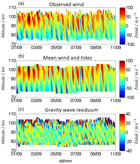
https://www.ann-geophys.net/37/851/2019/angeo-37-851-2019-f01

Figure 1Decomposition of the observed wind (a) into the mean wind and tidal component (b), and the gravity wave residuum (c) for Andenes 1–11 September 2017. Note the different labels of the color bar.

Download

To illustrate the different components, Fig. 1 shows a decomposition of the observed wind (top) into the mean wind and tidal component (middle) and the GW residual (bottom). The decomposition is shown for the location of Andenes for 10 d. Further information and a more detailed description regarding the algorithm can be found in Sect. 2.

LTCs in the atmosphere are complex. They are influenced by several factors, including fluctuations in solar and geomagnetic activity, which in turn can induce changes in the neutral density together with changes in the zonally directed winds (e.g., Emmert et al., 2008; Stober et al., 2012), or by anthropogenic emissions of greenhouse gases, which affect the troposphere through increased heating and causing cooling in the upper atmosphere (e.g., Beig, 2011; Las̆tovic̆ka et al., 2012). Several studies have investigated LTCs based on radar measurements for the northern high and mid latitudes, e.g., Middleton et al. (2001), Portnyagin et al. (2004), Portnyagin et al. (2006), Keuer et al. (2007), Jacobi et al. (2008), Hoffmann et al. (2011), Iimura et al. (2011), and Jacobi et al. (2015). From these studies, meteor radar wind observations show for the last decade season-dependent results for the mid latitudes, with stronger eastward- and southward-directed tendencies during the autumn and winter and opposite tendencies during the spring (e.g., Jacobi et al., 2015). For high latitudes, the zonal wind shows a time-varying tendency with an overall eastward-directed wind during the winter and also an increase in the semidiurnal tidal amplitude. However, large differences are present among these studies, which are based on different measurement intervals and different latitudes (e.g., Iimura et al., 2011).

In this study, we present climatologies and the decadal variability of winds, tides, gravity waves, and planetary waves from the northern high-latitude location of Andenes and the mid-latitude locations of Juliusruh and Tavistock (Canadian Meteor Orbit Radar – CMOR). The data are described in Sect. 2 and the resulting climatologies and decadal climate variabilities for the wind are presented in Sect. 3 and for diurnal and semidiurnal tides, gravity waves, and planetary waves in Sect. 4, respectively. The wind and tidal response on an 11-year oscillation is described in Sect. 5. Section 6 concludes the paper.

2 Data

This study uses observations from three meteor radars (MRs), which are located at the polar latitude station of Andenes (69.3^∘ N, 16.0^∘ E; Norway), the Juliusruh mid-latitude location (54.6^∘ N, 13.4^∘ E; Germany), and the mid-latitude location of Tavistock, the Canadian Meteor Orbit Radar (CMOR, 43.3^∘ N, 80.8^∘ W; Canada).

The Andenes MR was installed in 2002 and was run with a 15 kW transmitter at 32.55 MHz until May 2008. In May 2008 the system was moved to a new location 4 km away from the original site. Later in 2009, the system was further upgraded to 30 kW transmitting power. In 2011 and 2012 the original antennas were updated and replaced. Since 2012 the system has run in a stable hardware configuration. However, the experiment settings also underwent some changes during this interval. From 2002 to 2015 (October) the radar ran an experiment with a pulse repetition frequency of 2096 Hz and a 3.6 km mono pulse using a 2 km range sampling. In October 2015 the experiment was changed and the system is now operated with a pulse repetition frequency of 625 Hz and transmits a 7 bit Barker code with 1.5 km range sampling.

The time series of the Juliusruh MR is a composite of several different radar systems. From 2002 to 2010 the OSWIN radar was operated in a meteor mode interleaved to its normal MST-radar observations at a transmitting frequency of 53.5 MHz. These measurements were conducted 118 km west of the later Juliusruh MR site. In November 2007 the Juliusruh MR started its operation as a dual-frequency radar at 32.55 and 53.5 MHz. The experiment settings were similar to the ones in Andenes between 2002 and 2015. From 2014 to 2015 the system underwent several modifications. First, the experiment settings were changed to run the 625 Hz pulse repetition frequency and a 7 bit Barker code with 1.5 km range sampling (Stober and Chau, 2015). From January 2014 until autumn 2014 the transmitter of the Juliusruh 32.55 MHz system was not operating and only the 53.5 MHz system was observing. In spring 2015 the Juliusruh 53.5 MHz radar ceased its operation and the Juliusruh 32.55 MHz system remained operational, but with an increased transmitting power of 30 kW. Since this last modification, the system has operated continuously in a stable hardware and experiment configuration.

The CMOR MR provides the longest and most homogeneous MR time series used in this study. The system has run in a more or less unchanged configuration since 2002 as a triple-frequency system (17.45, 29.85, and 38.15 MHz) near Tavistock, Canada. Observations are carried out with a pulse repetition frequency of 532 Hz using a 11 km mono pulse and 3 km range sampling. The 17 and 38 MHz radars each use a 6 kW transmitter; the 29 MHz system was upgraded from 6 to 12 kW in the framework of the CMOR2 upgrade in May 2009. In this study, we compiled one homogeneous wind data set involving all available data of the triple-frequency observations.

In this study, the composites and LTCs are based on data sets for the years 2002–2018 for each location. The winds are obtained by applying a modified version of the all-sky fit (Hocking et al., 2001; Stober et al., 2018), and they have an hourly temporal resolution and partly cover the heights between 70 and 110 km, with a vertical altitude resolution of 2 km. The different atmospheric waves are extracted by an ASF (Stober et al., 2017; Baumgarten et al., 2018). In this study, we focus on observed mean winds, tides, gravity, and planetary waves. The statistical uncertainties are based on the applied fitting procedure by taking into account full error propagation of the radial wind errors as well as the number of meteors per altitude and time bin. The resulting uncertainties of the wind vary in the range of 2–16 m s⁻¹, with larger errors occurring in bins with fewer meteors or at the upper and lower edges of the meteor layer. More information about the experimental setup and the technical specifications for the Andenes and Juliusruh meteor radars, as well as about the wind analysis and the obtained uncertainties for all three radars, can be found in Stober et al. (2017, 2018). More technical information about CMOR and CMOR2 is described in, e.g., Webster et al. (2004), Jones et al. (2005), and Brown et al. (2008).

2.1 Homogenization of time series

The instruments used in this study were operational for almost 2 decades and some meteor radars did undergo substantial maintenance and modifications on the hardware. Most crucial for the wind measurements are the phase calibration and stability, the range sampling, and the Doppler measurement. The Andenes and Juliusruh meteor radars were maintained twice a year, including a test of the phase match of the cables and antennas. Further, the SKiYCORR software runs a phase test and provides a summary file of the impedance for each channel and day indicating potential problems. In addition to the regular maintenance, the CMOR meteor radar interferometry (phases) is cross-validated to optical observations. In particular, meteor showers are monitored with CMOR throughout the year, providing another source of information on the phase stability. The Andenes and Juliusruh meteor radars were also checked and cross-validated using selected meteor showers during the course of the year.

Both European meteor radars were frequently range and power calibrated using a delay line (Latteck et al., 2008; Stober et al., 2010). The CMOR radar is also routinely checked for potential issues in the range sampling by applying various cross-calibrations. All systems used the same software package over the complete time span to derive the Doppler velocities to avoid artefacts due to changes in the parameter estimation (e.g., Doppler velocity or the velocity uncertainty).

Before the multi-frequency data sets for CMOR and Juliusruh are compiled, we analyze the winds for each frequency independently and cross-validate the resultant time series. If one instrument shows systematic issues in the wind time series compared to the other instruments and the climatology, these data are flagged and are no longer considered in the finally compiled and merged wind time series. The Andenes meteor radar data are campaign-wise cross-validated with other meteor radars in Norway.

2.2 Adaptive spectral filtering of time series

The ASF provides a wave decomposition of our original observed time series into a daily mean wind, diurnal and semidiurnal tides, as well as a gravity wave residuum with an hourly resolution. Here, the gravity wave residuum also includes the terdiurnal tidal component. The hourly resolved time series are then averaged to daily means keeping the error information. The ASF is designed to account for the intermittency of waves, in particular, of tides and mean winds for time periods less than a day. Therefore, we adapt the window length of the harmonic tidal fit to the number of wave cycles. In the first step, we fit the daily mean wind with a window length of 24 h plus all tidal components. The next step uses the daily mean wind and the diurnal tidal component as a boundary to extract the information of the semidiurnal tide and so forth. This procedure is applied as a sliding window along the time series and all wave information (amplitude and phase) for all waves is determined for each time step. The technique is least squares based and, hence, robust against unevenly sampled data or data gaps shorter than the length of the window. Another benefit of the least squares implementation is the error propagation to all derived parameters. Further, we implemented a regularization constraint for the mean winds and diurnal and semidiurnal tides making use of the vertical wavelength information assuming that the mean winds and tidal phase should only show gradual changes within a vertical kernel function of 8 km for the mean winds and 10 km for the tidal phases. The daily mean wind time series (tides and gravity waves removed) are further analyzed to obtain the planetary wave activity. Therefore, we define a seasonal background wind based on the daily mean time series of u₀ and v₀ for the zonal and meridional components, respectively:

\begin{matrix} (3) & \begin{aligned} u_{0}, v_{0} & = u_{m}, v_{m} + \sum_{i = 1}^{2} a_{n} \sin (2 π / T_{n} \cdot t) \\ + b_{n} \cos (2 π / T_{n} \cdot t) . \end{aligned} \end{matrix}

Here u_m and v_m are an annual mean zonal and meridional wind, and a_n and b_n are coefficients for the seasonal subharmonics with periods $T_{n} = 365.25 / n$ d ( $n = 1, 2$ ). We determine the background wind field for every month at the 15th by fitting the above-described seasonal model to the daily mean wind time series using a 2-year window centered at the respective month and reconstruct the background wind time series for the other days for each month. The planetary wave activity is then given by subtracting the previously obtained daily mean winds and the reconstructed background wind field. The benefit of this approach compared to other techniques, e.g., smoothing the data or running averages, is that it is more robust against larger data gaps of up to months in length. Another benefit is that, due to the long window used for the fitting, seasonal peculiarities, e.g., sudden stratospheric warmings, do not affect the monthly means, but are well captured in the planetary wave activity.

Monthly mean tidal amplitudes and GW and PW activity are derived by computing monthly medians of the available data sets. Thus, the resultant time series contain some data gaps. However, there are still enough data points to estimate a LTC and a potential solar cycle effect for all these waves for each month. The LTC and solar cycle effect are derived by using a linear trend model plus an 11-year oscillation, which is not tied to the F10.7 solar radio flux or the sunspot number. Qian et al. (2019) analyzed WACCM-X and wind observations above Collm (51^∘ N, 13^∘ E) and found that the wind signature is less statistically significant than the temperature response to the solar radio flux. Other studies exploring the stratospheric/tropospheric response to solar forcing indicate a clearer dependence (Salby and Callaghan, 2006; Rind et al., 2008; Lu et al., 2017) on solar activity. At the MLT, the wind seems to be less directly influenced by the F10.7 or sunspot number. Pokhotelov et al. (2018) found almost no correlation between the occurrence of mesospheric echoes at mid latitudes and the solar radio flux (F10.7), but a clear dependence on the occurrence of these echoes due to meridional winds. Further, Stober et al. (2014) investigated the neutral air density response during solar cycle 23 and found a phase delay of almost 1 year between the F10.7 proxy and the neutral air density variation. Considering all the aspects above, we model the resulting mean winds as

\begin{matrix} (4) & \begin{aligned} u_{mm}, v_{mm} & = a_{u, v} + m_{u, v} \cdot t + a \cdot \sin (2 π / 11.0 \cdot t) \\ + b \cdot \cos (2 π / 11.0 \cdot t), \end{aligned} \end{matrix}

where u_mm and v_mm are the monthly mean zonal and meridional components for the mean wind and each wave, m_u,v is linear change over the whole period, a and b are the solar cycle components, a_u,v is the mean at year 0, and t is the time in years.

3 Climatologies and long-term changes in the mean wind

Analyzing long time series always requires an estimate of the associated confidence values of the measured linear changes or other derived parameters. In this study, we conduct a full error propagation to all parameters using the covariance matrices of the fitted functions. Based on this statistical uncertainty we are able to define the 90 % and 95 % confidence levels given by x±σz. Here x is a parameter, σ is the statistical uncertainty of x, and z is a factor, which takes values z=1.64 for the 90 % confidence interval and z=2 for the 95 % interval, respectively, assuming a Gaussian error distribution. We label the different confidence intervals by dashed (90 %) and solid (95 %) contours for all derived parameters. We tested our confidence intervals for whether they are significant by introducing two null hypotheses. The long-term linear changes are tested under the assumption that there is no linear change as a null hypothesis, and the solar cycle is tested with the null hypothesis that there is no significant solar cycle. However, it is also important to note that there could be a potential autocorrelation in our time series due to the solar cycle. We estimated all confidence levels under the assumptions that the Gauss–Markov theorem holds and our least square estimators are an unbiased solution, viz. that the fit residuals are uncorrelated.

Mean wind climatologies at the MLT are often shown for a particular location or instrument or as averages over different periods. In this study we present climatologies of mean winds, diurnal and semidiurnal tides, and PW and GW activity covering more than 25^∘ latitude from mid latitudes to polar latitudes. Thus we are providing a profile of the mean wind systems at the MLT over the Northern Hemisphere. Furthermore, the data sets span the same observational periods from 2002 to 2018 and the winds are obtained by the same type of analysis.

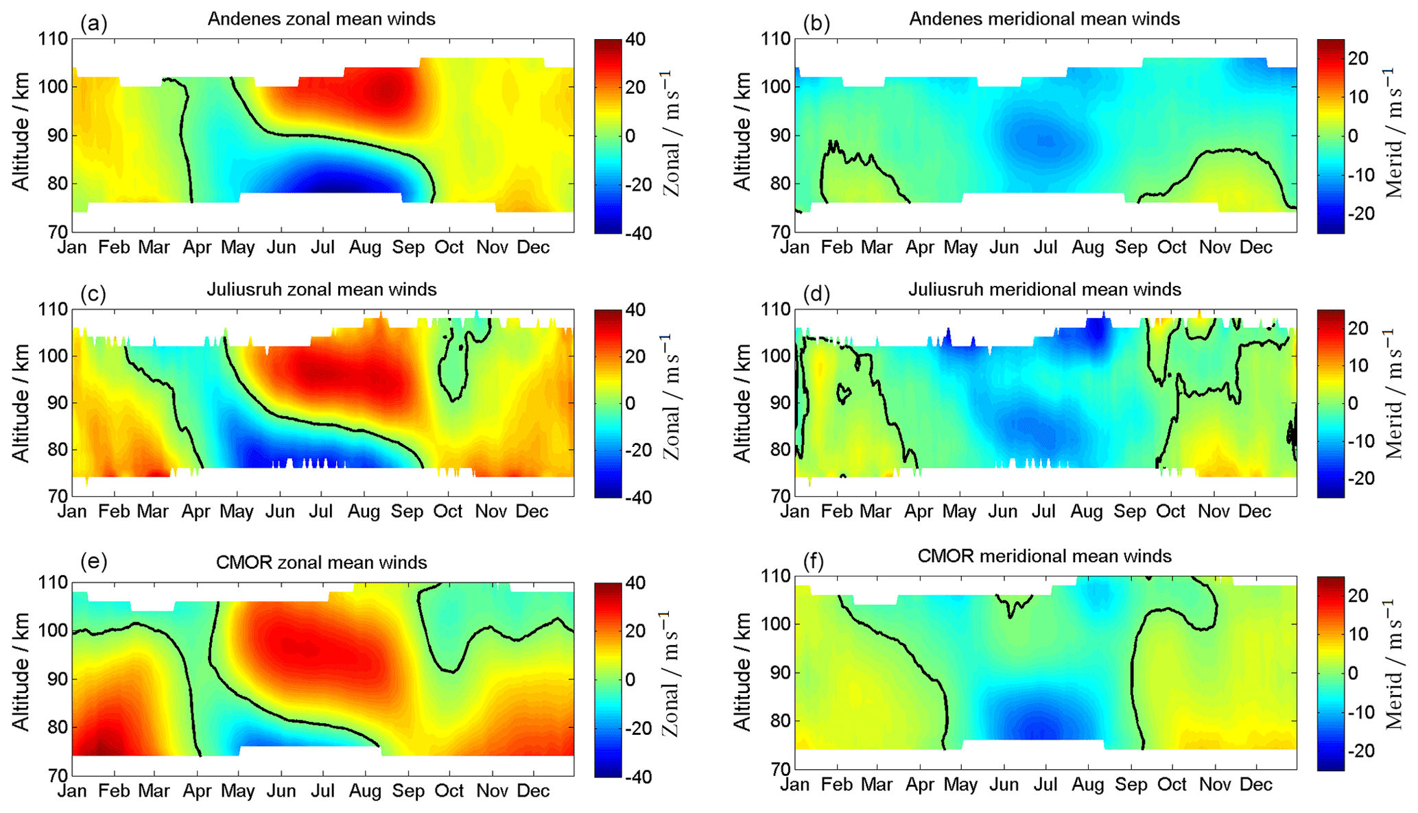
https://www.ann-geophys.net/37/851/2019/angeo-37-851-2019-f02

Figure 2Composite of zonal (a, c, e) and meridional (b, d, f) wind components for Andenes (a, b), Juliusruh (c, d), and CMOR (e, f). The black line corresponds to the wind reversal. Note the different labels of the color bar.

Download

The mean wind climatologies are shown in Fig. 2. Every location shows a distinct seasonal pattern, with eastward-directed winds during the winter and a transition/reversal between eastward and westward winds during the summer. Meridional winds are northward-directed during the winter and southward-directed during the summer. The zero line transition is shown as a black contour line. The zonal wind pattern indicates two pronounced features when comparing the different latitudes. In winter, the eastward-directed winds are much stronger at CMOR, with up to 40 m s⁻¹, and decrease towards higher latitudes with 6–10 m s⁻¹. Further, CMOR shows a zero line crossing in the zonal winds around 100 km altitude, which is not seen at Juliusruh and Andenes. During the fall transition, Juliusruh shows for a month at altitudes above 95 km westward-directed wind. During summer the wind pattern looks rather similar; just the zonal wind reversal altitude increases from the mid latitudes towards the polar latitudes by almost 8–10 km (June, July, August).

The meridional wind climatology also shows latitudinal differences. During the winter season, the mid latitudes show northward winds of magnitude 10 m s⁻¹. The summertime is characterized by a southward mesospheric jet of 10–15 m s⁻¹, which is closely related to the zonal wind reversal. The most prominent features in the meridional winds are the zero line and its altitude variation during the course of the year. At Andenes, northward winds occur only below 90 km altitude and then for only a few months in winter. In contrast, at the mid-latitude stations northward winds are found at all altitudes throughout the winter and southward winds for the summer months. Due to the different lengths of time series compared to other studies, these results are only partly consistent with findings of, e.g., Yuan et al. (2008 b), Kishore Kumar and Hocking (2010), Hoffmann et al. (2011), Jacobi (2012), Conte et al. (2018), and Lukianova et al. (2018).

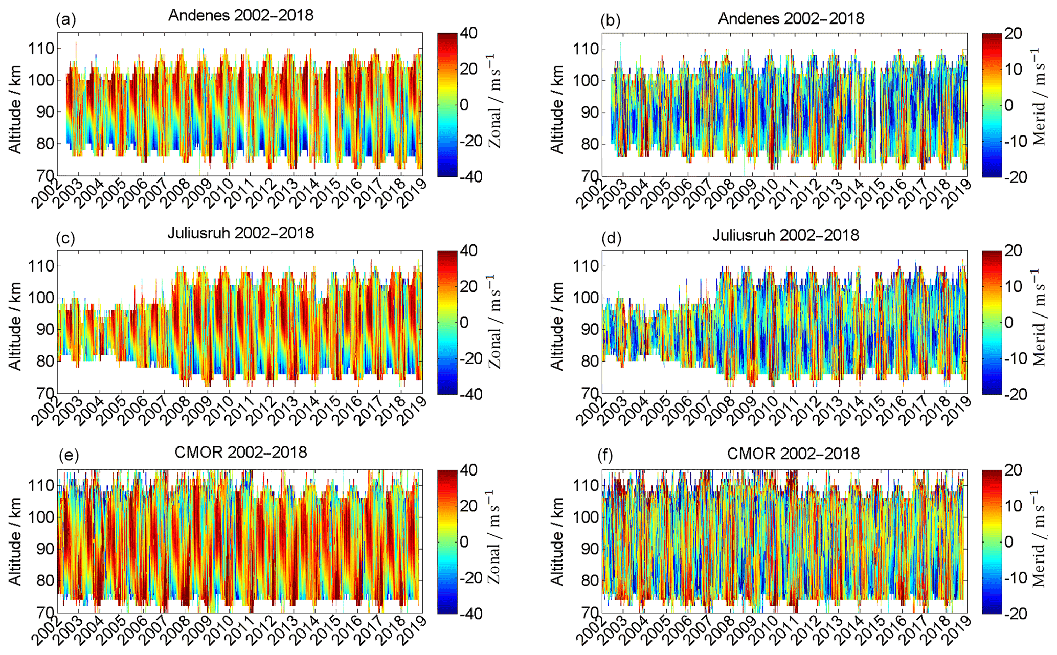
https://www.ann-geophys.net/37/851/2019/angeo-37-851-2019-f03

Figure 3Observed zonal (a, c, e) and meridional (b, d, f) wind components for Andenes (a, b), Juliusruh (c, d), and CMOR (e, f) for the locations according to available data series. Note the different labels of the color bar.

Download

Although the climatologies are statistically robust regarding the mean patterns in both wind components, there is a year-to-year variability and also changes over much longer timescales. Figure 3 shows the time series of the zonal (left) and meridional (right) winds for the Andenes high-latitude location (top) and the Juliusruh (middle) and CMOR (bottom) mid-latitude locations. As described in Sect. 2, especially for Juliusruh, the system modifications resulted in an increase in the altitude coverage due to software and hardware improvements over several years. The seasonal pattern, shown in the climatologies (Fig. 2), is even more clearly visible in Fig. 4, where the year-to-year variability is more pronounced, by using the seasonal fit removing the PW activity from the time series.

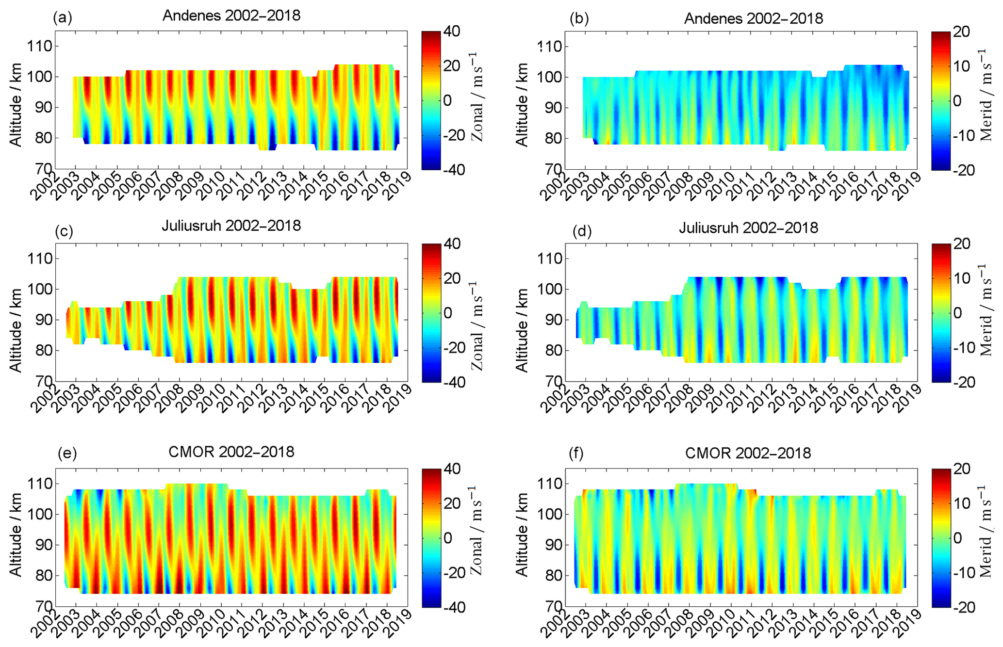
https://www.ann-geophys.net/37/851/2019/angeo-37-851-2019-f04

Figure 4Seasonal mean zonal (a, c, e) and meridional (b, d, f) wind components for Andenes (a, b), Juliusruh (c, d), and CMOR (e, f) for the locations according to available data series. Note the different labels of the color bar.

Download

Just by visual inspection of Fig. 4, some of the year-to-year variability or LTC becomes visible; e.g., for the years 2003–2007 CMOR shows a westward-directed wind regime above 100 km during summer, which disappears in more recent years. Furthermore, there is an enhancement of the southward-directed winds in Andenes after the year 2015 at altitudes above 95 km.

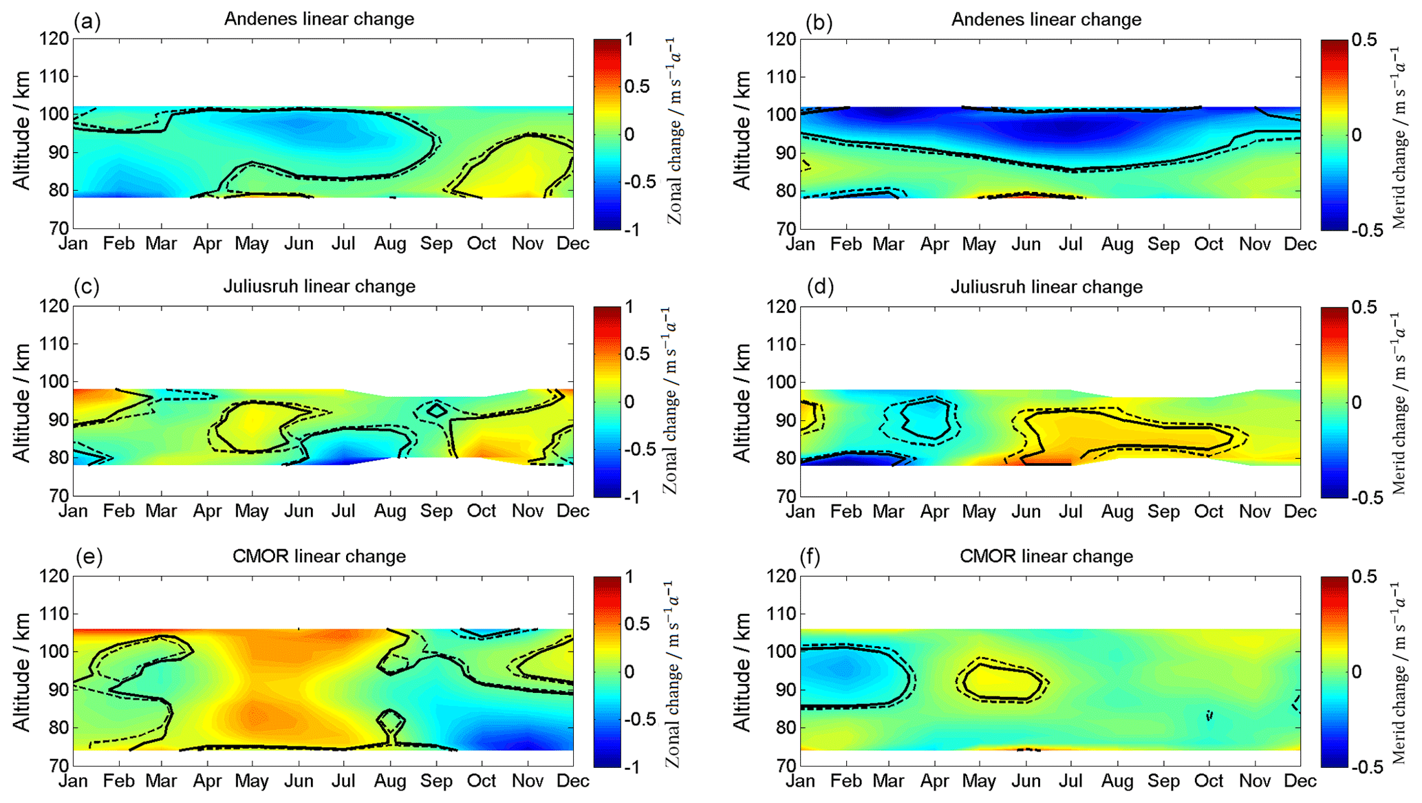
https://www.ann-geophys.net/37/851/2019/angeo-37-851-2019-f05

Figure 5Linear long-term changes in zonal (a, c, e) and meridional (b, d, f) wind for Andenes (a, b), Juliusruh (c, d), and CMOR (e, f). Note the different labels of the color bar. The solid black lines correspond to the 95 % significance, the dashed black lines to the 90 % significance.

Download

Monthly changes are estimated using Eq. (4) and are shown in Fig. 5 for both wind components. The dashed black lines represent the 90 % confidence level and the solid black lines the 95 % confidence level. It is rather obvious from Fig. 5 that there is no common linear change at all three latitudes, and thus we discuss each site separately. At Andenes, an enhancement of the westward-directed wind occurs during the beginning of the year with values of up to 0.3 $m s^{- 1} {year}^{- 1}$ , as well as for the summer in the area above the transition height. After the fall transition, a small enhancement of eastward winds is found, with values of up to 0.3 $m s^{- 1} {year}^{- 1}$ below 100 km. The meridional wind for Andenes shows a pronounced southward-directed wind long-term variability, with values of up to 0.5 $m s^{- 1} {year}^{- 1}$ above ∼96 km for the winter and above ∼90 km for the summer. The LTC for Juliusruh is less significant, with changes which correspond to an eastward-directed tendency during the beginning of April and May and westward-directed below 90 km at June/July. Furthermore, eastward enhancements below 90 km between September and November and at the beginning of the year above 90 km, with values of up to 0.5 m s⁻¹, are found. The meridional component of Juliusruh shows tendencies towards south between January and April and an opposite tendency between May and November. At the location of CMOR, the strongest significant LTC occurs between April and August with an eastward acceleration of the zonal wind, enhancing the zonal jet above 90 km and weakening the westward jet below with values of up to 0.5 $m s^{- 1} {year}^{- 1}$ . Meridional winds at CMOR show a southward long-term variability between 90 and 100 km at the beginning of the year and some northward accelerations in summer.

https://www.ann-geophys.net/37/851/2019/angeo-37-851-2019-f06

Figure 6Linear long-term changes in zonal (red) and meridional (blue) wind, based on annual values for Andenes (a), Juliusruh (b), and CMOR (c). The error bars correspond to the statistical variance.

Download

The seasonal analysis provides information about the mean zonal and meridional wind for each year and altitude. Figure 6 shows the vertical LTC based on annual mean values. The vertical profiles indicate the linear change per decade of the zonal (red) and meridional (blue) wind. The most significant changes occur at Andenes in both wind components. The mean zonal wind speed is decreasing between 85 and 100 km by up to 3 $m s^{- 1} {decade}^{- 1}$ . The LTC of the meridional wind reaches values up to 2 $m s^{- 1} {decade}^{- 1}$ . At mid latitudes (Juliusruh) the zonal wind shows only a weak change per decade and an eastward acceleration with 0–0.5 $m s^{- 1} {decade}^{- 1}$ . The meridional winds indicate a more pronounced linear tendency. Below 85 km the meridional jet seems to be further westward accelerated, whereas at higher altitudes an eastward acceleration is found. At CMOR the zonal wind shows almost no long-term variability at all altitudes between 75 and 110 km. The meridional wind indicates a LTC above 90 km altitude corresponding to a northward acceleration of the mean circulation.

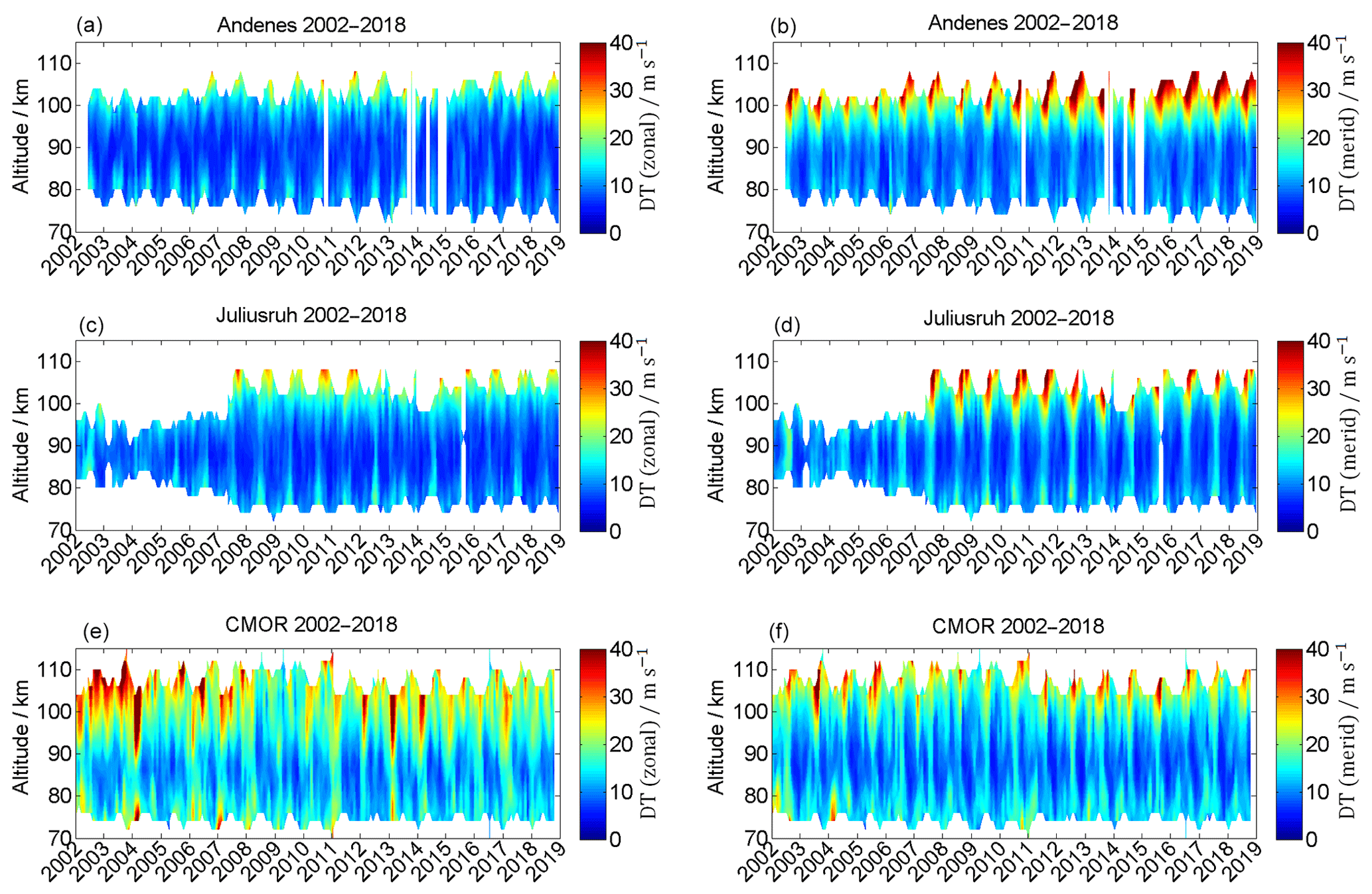
https://www.ann-geophys.net/37/851/2019/angeo-37-851-2019-f07

Figure 7Time series of the zonal (a, c, e) and meridional (b, d, f) diurnal tidal components for Andenes (a, b), Juliusruh (c, d), and CMOR (e, f).

Download

https://www.ann-geophys.net/37/851/2019/angeo-37-851-2019-f08

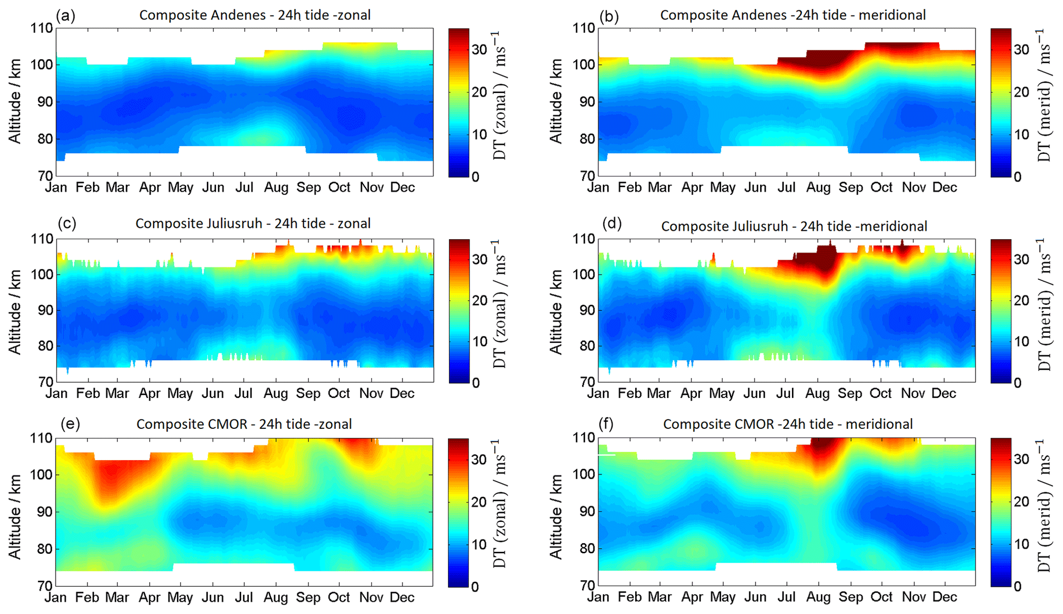
Figure 8Composites of the zonal (a, c, e) and meridional (b, d, f) diurnal tidal components for Andenes (a, b), Juliusruh (c, d), and CMOR (e, f).

Download

4 Climatologies and long-term changes in waves

4.1 Diurnal tides

The monthly median amplitudes and the associated composites for the tidal 24 h diurnal components are shown in Figs. 7 and 8. The seasonal pattern of the diurnal tidal (DT) amplitude shows a rather rapid increase around 100 km altitude and at least during the summer a secondary enhancement around 80 km altitude with values of ∼15 m s⁻¹. Comparing all three locations, CMOR shows the strongest maximum and strongest mean amplitudes for the zonal diurnal tides, with mean values larger than 25 m s⁻¹. This occurs at heights above 90 km and especially between January and April shows a general enhancement of the zonal diurnal tidal amplitude. Juliusruh reaches maximum mean values of ∼25 m s⁻¹ only between the late summer and autumn above 100 km. During this time, Andenes also shows the strongest diurnal tidal amplitudes in the zonal direction, but with weaker maximal mean values of up to 20 m s⁻¹. The meridional diurnal tidal component at all three locations shows a similar pattern, with enhancements of the amplitudes between summer and winter, for heights above 94 km, where it reaches maximum mean values of over 30 m s⁻¹. All locations show a second increase during the summer around 82 km, and even higher up for CMOR, with mean values of 15–20 m s⁻¹. Another very prominent feature of the diurnal tidal amplitudes is related to its polarization relation. At Andenes and Juliusruh the meridional component is significantly enhanced compared to the zonal diurnal tidal amplitude. At CMOR this effect is less pronounced during June–December and reverses in spring, where the zonal diurnal tidal amplitude is much larger compared to the meridional component.

Comparing our climatologies to previous studies reveals some interesting differences. Portnyagin et al. (2004) and Jacobi (2012) found a distinct maximum during the summer months and almost no tidal signature in winter at altitudes from 92 to 98 km. Both studies also did not show the diurnal summer maximum below 82 km. These differences are partly explainable by the different length of the analyzed time series. Portnyagin et al. (2004) could only use a bit more than 1 year of data for the Scandinavian climatology. Jacobi (2012) compiled a climatology from 6 years during solar minimum conditions. However, the ASF decomposition of tides and mean winds considering the intermittent behavior of the diurnal amplitude and phase may also play a role.

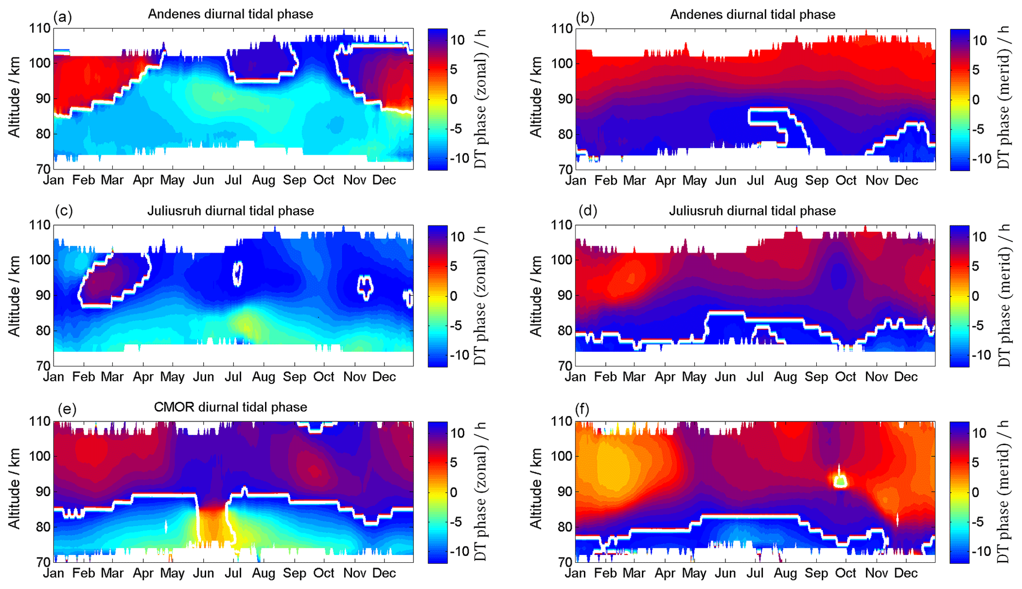
https://www.ann-geophys.net/37/851/2019/angeo-37-851-2019-f09

Figure 9Composites of the zonal (a, c, e) and meridional (b, d, f) diurnal phase information for Andenes (a, b), Juliusruh (c, d), and CMOR (e, f).

Download

The diurnal tidal phases are shown in Fig. 9. The phases are referenced to a longitude of 13^∘ east. The white contour line labels phase jumps and zero phases. The CMOR phases are shifted as if they would have been observed at the CMOR latitude but at the above-mentioned longitude in the European sector. The diurnal tidal phases show a distinct seasonal pattern and latitudinal differences. Throughout the year there are substantial changes in the phases at a given altitude; in particular, at the polar latitudes during the winter months, the phases undergo phase drifts of several hours within a month.

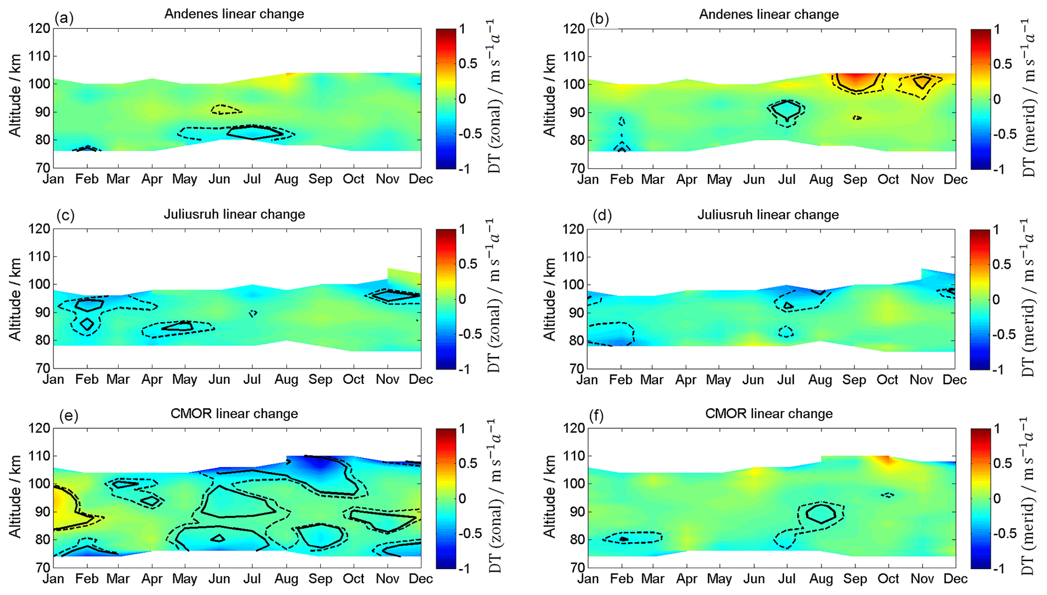
https://www.ann-geophys.net/37/851/2019/angeo-37-851-2019-f10

Figure 10Linear long-term changes in zonal (a, c, e) and meridional (b, d, f) diurnal tidal components for Andenes (a, b), Juliusruh (c, d), and CMOR (e, f). The solid black lines correspond to 95 % significance, the dashed black lines to the 90 % significance.

Download

Based on the long-term series, Fig. 10 indicates the interannual LTC for the diurnal components. For the locations of Andenes and Juliusruh, the diurnal component shows small but significant tendencies. During the summer at Andenes, a westward-directed amplitude gradient is present in the westward wind regime below 85 km, with values of up to 0.3 $m s^{- 1} {year}^{- 1}$ . Furthermore, there is a northward-directed wind amplitude change during the fall at around 100 km. At the location of Juliusruh, changes take place in the zonal component during the winter, with a tendency towards a decreasing diurnal tidal activity above 90 km. However, at Andenes and Juliusruh the zonal and meridional diurnal tidal amplitudes show only rather small changes from 2002 to 2018. At CMOR changes emerge between 82 and 100 km in January. During the early winter, the LTC shows an increasing diurnal tidal amplitude activity, with values up to 0.4 $m s^{- 1} {year}^{- 1}$ for the zonal component and almost no change for the meridional component. During the summer months, the LTC points towards a decreasing tidal amplitude, with up to 1 $m s^{- 1} {year}^{- 1}$ for heights above 100 km. Meridional tidal diurnal amplitudes at CMOR exhibit only small changes.

https://www.ann-geophys.net/37/851/2019/angeo-37-851-2019-f11

Figure 11Same as Fig. 7 but for the semidiurnal tidal components.

Download

https://www.ann-geophys.net/37/851/2019/angeo-37-851-2019-f12

Figure 12Same as Fig. 8 but for the semidiurnal tidal components.

Download

4.2 Semidiurnal tides

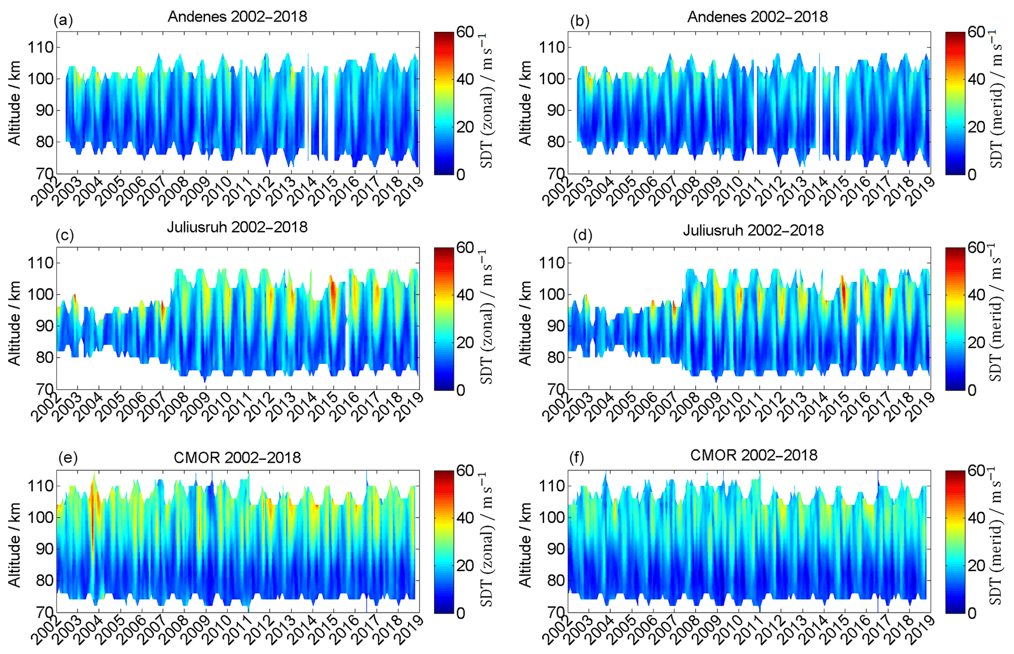
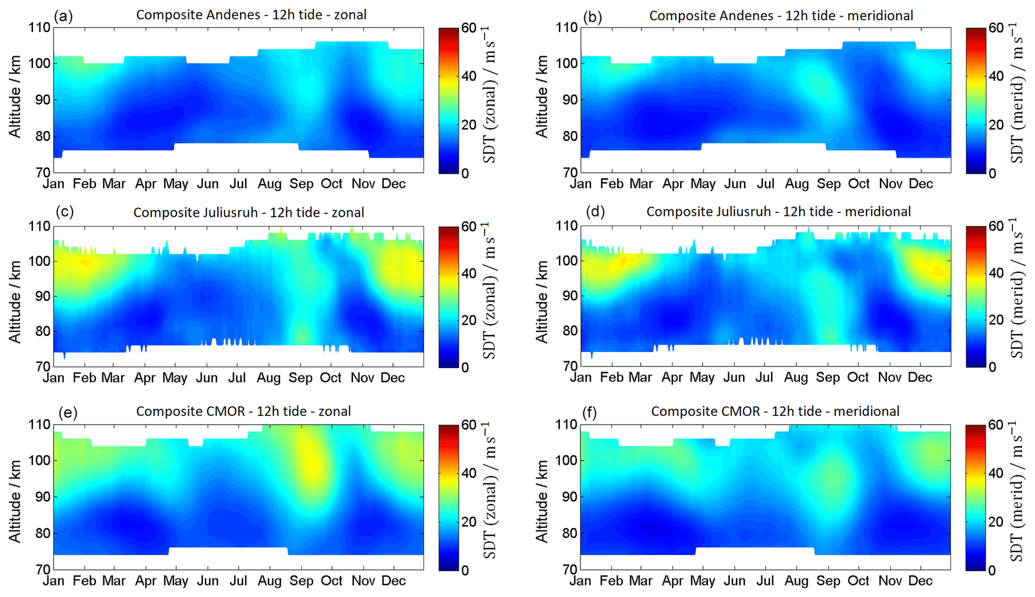
The 12 h semidiurnal tide is the most dominant wave in the MLT throughout the year at mid and high latitudes. The time series of semidiurnal tidal (SDT) amplitudes is presented in Fig. 11 and the SDT climatology is given in Fig. 12. SDT amplitudes are usually larger compared to DT amplitudes and reach at the mid latitudes for the zonal wind component maximum mean values of ∼30–40 m s⁻¹ and for the meridional component maximum mean values of 20–40 m s⁻¹. In general, the semidiurnal tidal components at all locations show similar seasonal patterns. SDT amplitudes increase with increasing heights and reach maximum values around 100 km altitude. The seasonal pattern of the SDT shows a very similar morphology throughout the year at all three MR sites. There is a winter maximum, a spring minimum, and a second amplification during September–October and a second minimum in November. At Andenes the SDT amplitude reaches mean values for both components of up to 30 m s⁻¹. The highest SDT amplitudes are seen at mid-latitude station Juliusruh during the winter months, with values of up to 40 m s⁻¹. In contrast, the fall transition reaches its highest SDT amplitudes of ∼40 m s⁻¹ (zonal component) at CMOR.

At Andenes and Juliusruh the zonal and meridional wind components indicate similar values for amplitudes and occurrence of the SDT. Comparable amplitudes are present during the winter months at CMOR. However, the fall transition above looks slightly different for the CMOR MR. The zonal SDT amplitude appears to be larger than the meridional component.

https://www.ann-geophys.net/37/851/2019/angeo-37-851-2019-f13

Figure 13Same as Fig. 9 but for the semidiurnal tidal components.

Download

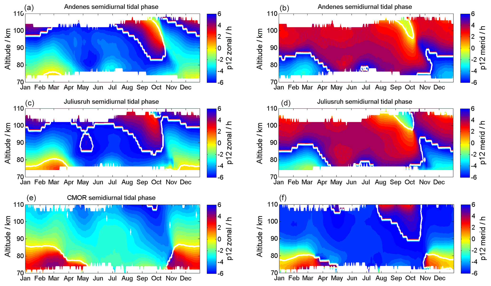
Figure 13 shows the phase behavior for the SDT. The seasonal pattern indicates an asymmetry and rapid phase change during the fall transition and the winter months. During the spring transition the phases also are altered, but are less prominent compared to the fall and winter time. The phases also reflect the seasonal asymmetry similar to the amplitudes of the SDT. Further, it appears that latitudinal differences between Andenes and Juliusruh are small, whereas the phase differences to the CMOR latitude are much more significant. SDT phases also show continuous phase changes throughout the year. During the fall transition the phase changes within a month by more than 6 h at all three latitudes. However, the winter time is also characterized by drifting SDT phases within a month.

https://www.ann-geophys.net/37/851/2019/angeo-37-851-2019-f14

Figure 14Same as Fig. 10 but for the semidiurnal tidal components.

Download

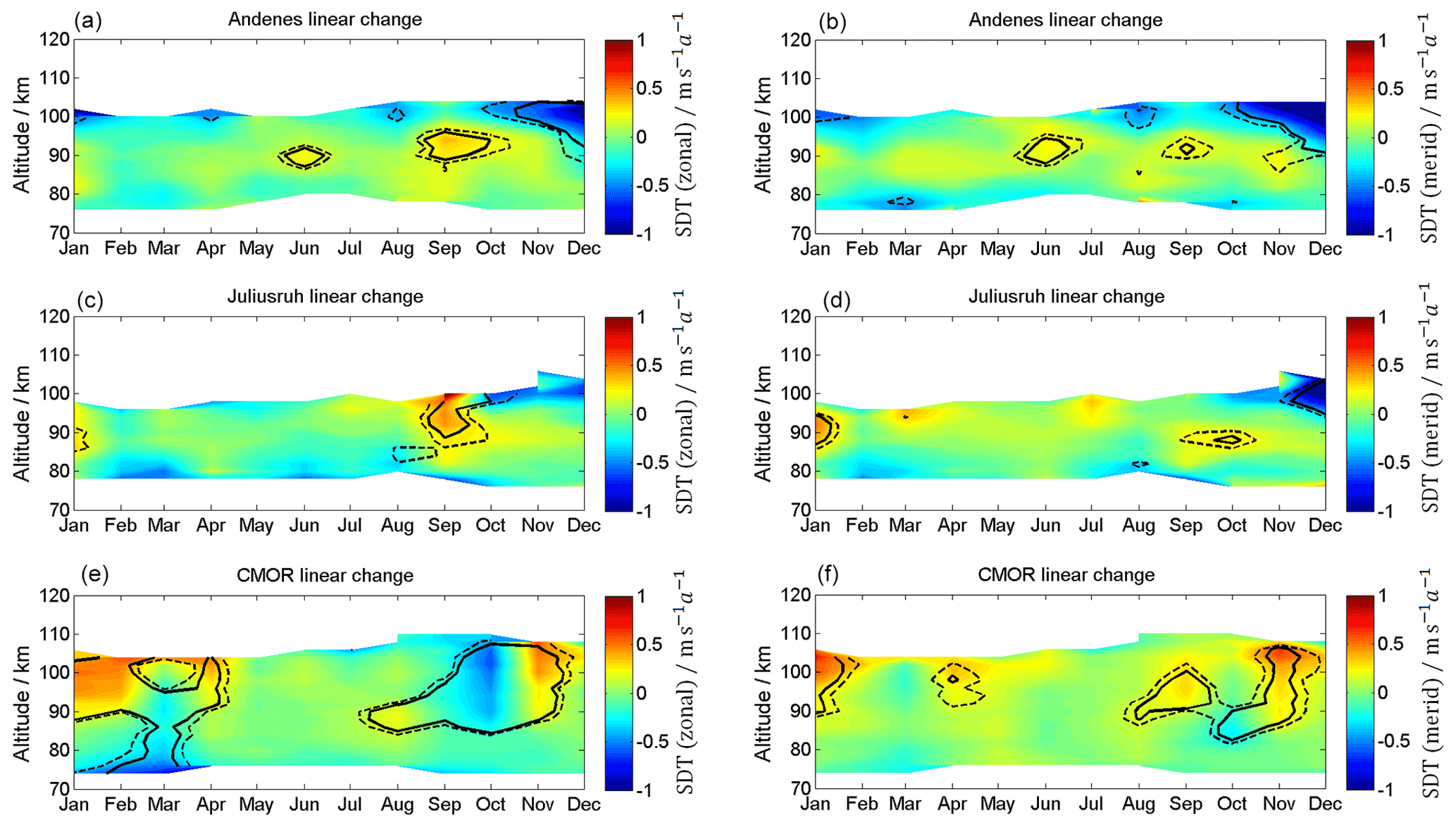
The LTC for the semidiurnal tides is shown in Fig. 14. At Andenes a significant change emerges above 90 km during the winter (November, December), showing a rather strong decrease in the SDT with amplitudes of 1 $m s^{- 1} {year}^{- 1}$ . Additionally, a significant enhancement of the SDT occurs during the autumn transition, showing an increase of up to 1 $m s^{- 1} {year}^{- 1}$ . Similar patterns for the summer also occur for Juliusruh. This behavior is not reflected at CMOR. There, it appears that the SDT amplitudes in November are further increasing in the zonal and meridional components. CMOR also exhibits a significant increase in the wintertime (December–February) of SDT amplitudes above 90 km.

https://www.ann-geophys.net/37/851/2019/angeo-37-851-2019-f15

Figure 15Time series of planetary wave energy for Andenes (a), Juliusruh (b), and CMOR (c). The red (green) bold arrows correspond to winter with a major (minor) sudden stratospheric warming.

Download

4.3 Planetary and gravity waves

The planetary wave activity is estimated as residual between the daily mean winds, as obtained from the adaptive spectral filtering and the seasonal fit shown in Eq. (3). The seasonal fit provides a robust estimate of a background wind field for every day of the year and each wind component. The zonal and meridional wind residuals can be written as u^′ and v^′ and are considered a good proxy of a planetary wave amplitude. However, this method does not allow us to distinguish between a planetary-wave-like oscillation and a SSW event, which typically lasts 3–5 d at the MLT. However, Matsuno (1971) already pointed out that PWs play a major role in the evolution of SSWs. Figure 15 shows the PW energy. All three locations show striking enhancements during the winter, especially during years when a major sudden stratospheric warming (red arrow) takes place. During the years with a major sudden stratospheric warming event, the PW energy appears to be increased and takes values of up to 300 m² s⁻² in the winter months. Minor sudden stratospheric warmings (green arrow) show also an increase in the PW energy, but are usually weaker than during years with a major sudden stratospheric warming. Even for the year 2016, where we found an exceptional circulation pattern at the MLT, an enhancement of the PW energy is present Stober et al. (2017), although this year did not show the evolution of a typical SSW (Matthias and Ern, 2018). For the rest of the year, the PW activity is comparatively low, with sparse enhancements observed at CMOR.

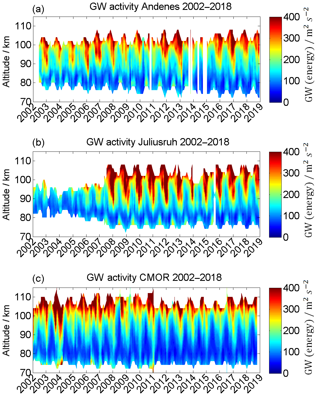
https://www.ann-geophys.net/37/851/2019/angeo-37-851-2019-f16

Figure 16Time series of kinetic gravity wave energy for Andenes (a), Juliusruh (b), and CMOR (c).

Download

https://www.ann-geophys.net/37/851/2019/angeo-37-851-2019-f17

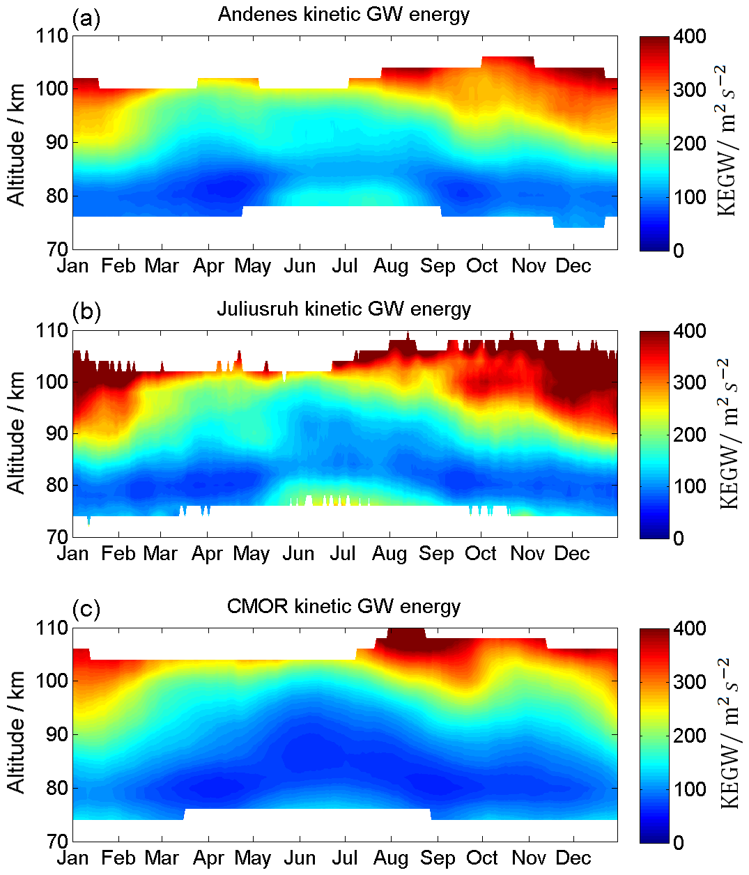
Figure 17Composite of kinetic gravity wave energy for Andenes (a), Juliusruh (b), and CMOR (c).

Download

In Figs. 16 and 17 the long-term observations of kinetic gravity wave energy (GW) and the corresponding GW energy climatology are presented. The general seasonal pattern for all three locations appears to be quite similar. An enhancement of the kinetic GW energy with increasing heights is noticeable, as well as a seasonal pattern with increased GW energies between the autumn transition and the end of the winter, with values of up to 400 m² s⁻². Below a height of ∼82 km during the summer there is a secondary enhancement, which is especially noticeable at Andenes and Juliusruh. At that time, values of up to ∼150 m² s⁻² are recorded for Andenes, and up to ∼250 m² s⁻² for Juliusruh.

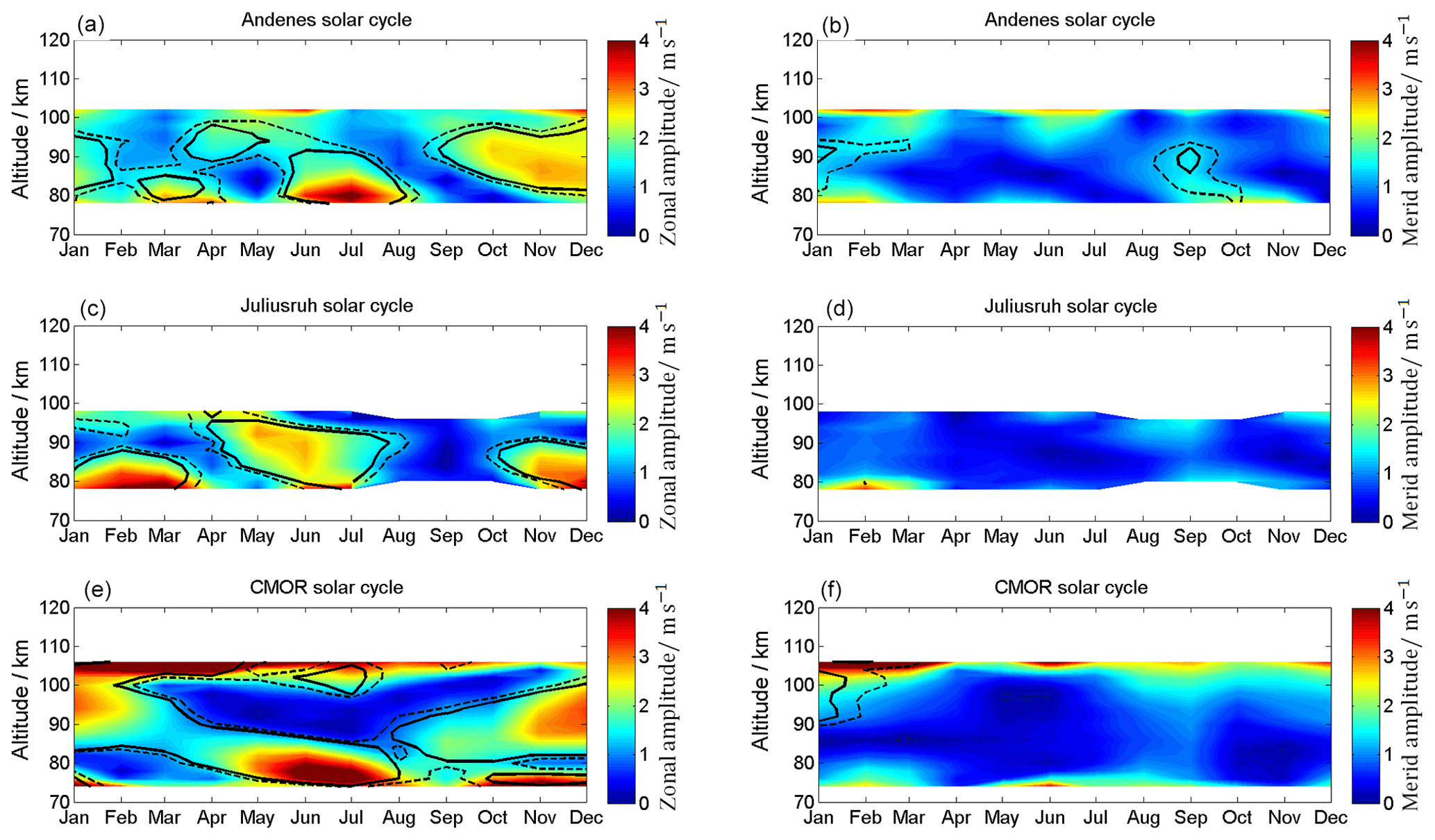
https://www.ann-geophys.net/37/851/2019/angeo-37-851-2019-f18

Figure 18Linear change in the solar radiation on the zonal (a, c, e) and meridional (b, d, f) wind for Andenes (a, b), Juliusruh (c, d), and CMOR (e, f). The solid black lines correspond to 95 % significance, the dashed black lines to the 90 % significance.

Download

5 Wind dependencies on an 11-year oscillation

For long-term wind data which exceed the period of a solar cycle it is advantageous to consider the influence of an 11-year oscillation on the wind. Figure 18 visualizes the impact of an 11-year oscillation on a seasonal basis. All three stations show nearly no changes in the meridional component, while the zonal winds appear to be highly responsive to the solar activity during the summer around 80 km and during the winter. At the equinoxes, the zonal wind component is unaffected by the 11-year modulation. During the summer, all three locations show an 11-year oscillation with an amplitude response between 3 and 5 m s⁻¹ below 82 km.

https://www.ann-geophys.net/37/851/2019/angeo-37-851-2019-f19

Figure 19Linear change in an 11-year oscillation on the diurnal zonal (a, c, e) and meridional (b, d, f) tidal components for Andenes (a, b), Juliusruh (c, d), and CMOR (e, f). The solid black lines corresponds to 95 % significance, the dashed black lines to the 90 % significance.

Download

https://www.ann-geophys.net/37/851/2019/angeo-37-851-2019-f20

Figure 20Same as Fig. 19 but for the semidiurnal component.

Download

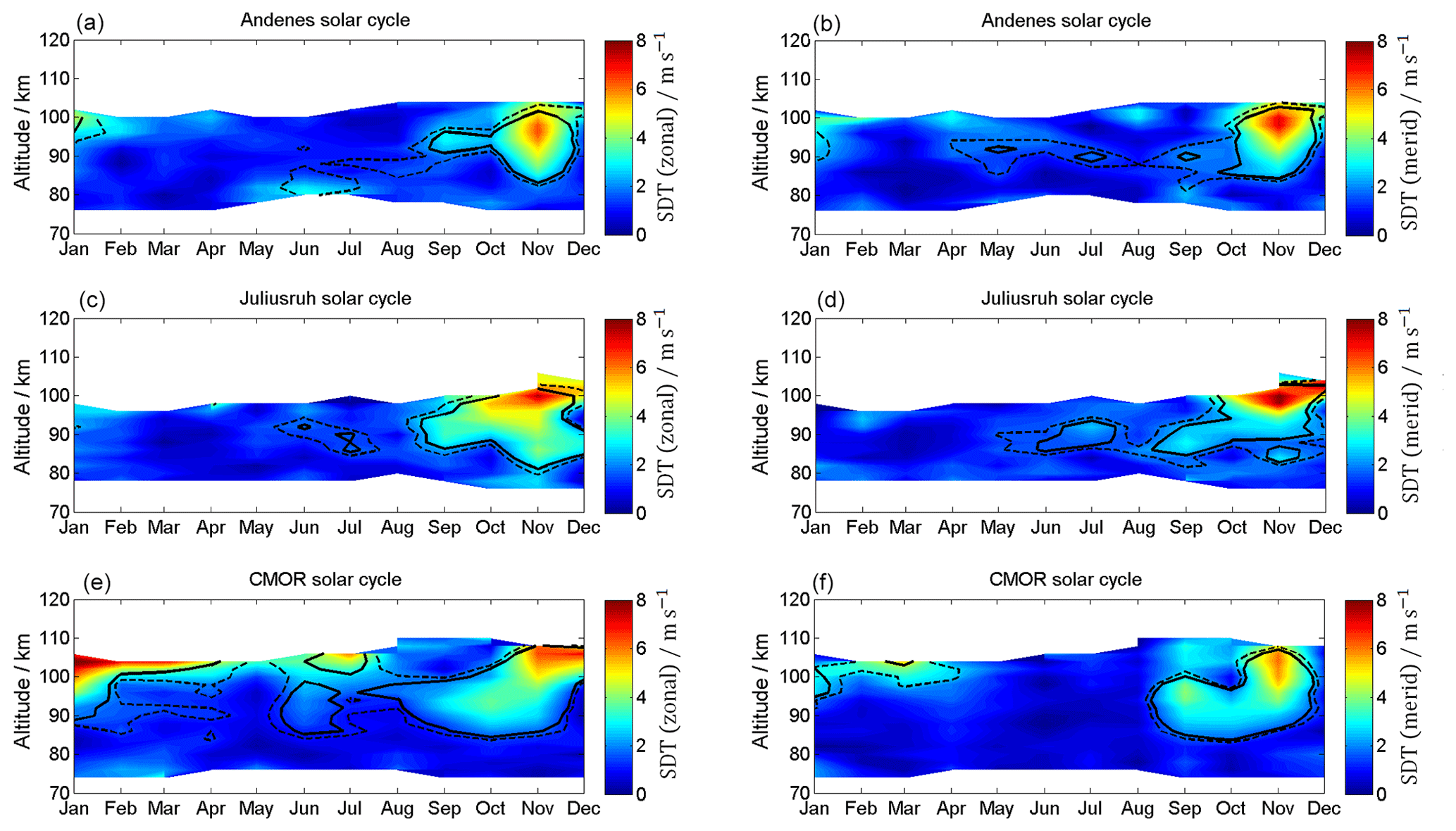
In addition to the annual profile, Figs. 19 and 20 show seasonal linear influences of solar radiation on the tidal components. The influence of the 11-year oscillation on the diurnal tides is shown in Fig. 19. Andenes and Juliusruh show no changes in the zonal component, while the 11-year oscillation in CMOR becomes prominent above 90 km. For the meridional component, only Andenes and CMOR are affected above 94 km during the summer months, by values of up to 4 m s⁻¹. For the semidiurnal tides (Fig. 20) all locations show for both components enhancements during and after the autumn transition above ∼90 km, which last at CMOR until the spring. These enhanced values are remarkable because during the time after the autumn transition the tidal amplitudes are quite low (see Fig. 12), which indicates an increased response to the solar cycle for this period of the year. The modulation of the semidiurnal tidal amplitudes due to the solar cycle forcing ranges between 3 and 6 m s⁻¹ for the winter season. Considering that some of the previous tidal climatologies are compiled during different phases of a solar cycle explains some of the discrepancies (Jacobi, 2012; Pokhotelov et al., 2018).

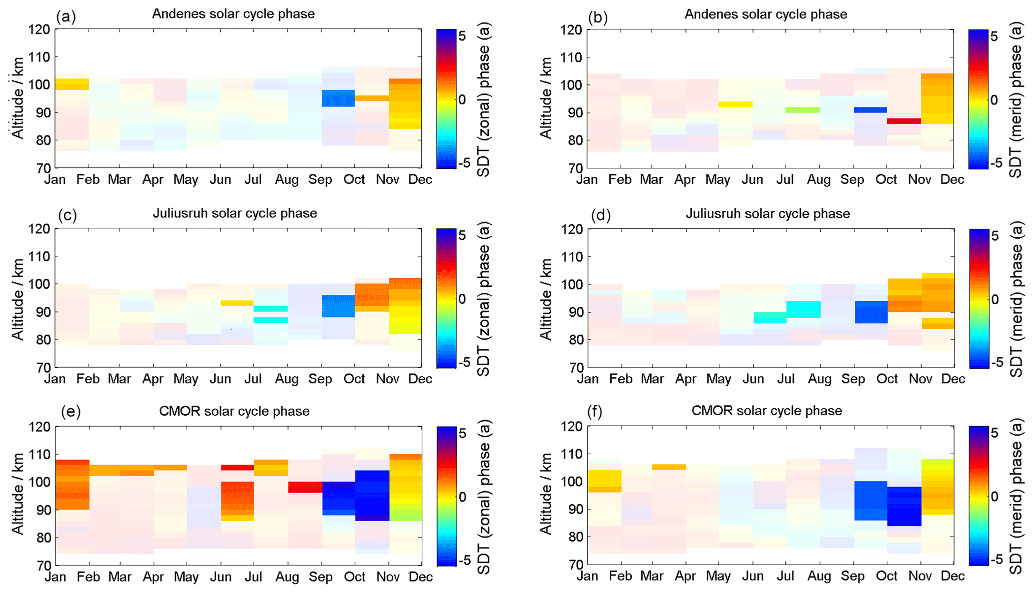
The phase information for the solar cycle can be found in the Appendix. The phase is referenced to the year 2002. The yellowish to light orange color indicates a zero phase shift compared to the reference year and corresponds to the maximum solar activity during solar cycle 23 (e.g., F10.7 or sunspot number). Phases that are outside the 90 % confidence interval are shaded and should not be treated as reliable due to the weak signal. The phase behavior itself seems to be rather complex and depends on season and altitude. The phase pattern of mean winds also shows a strong latitude dependence in both wind components. Only the winter season exhibits similarities in the response to the solar cycle of the sun with respect to the phase behavior. There is a certain coherence of the phases between the latitudes, in particular for the semidiurnal tide, which indicates a pronounced phase offset between September/October and December/January, which requires further investigation. However, the diurnal tide is basically only affected at the CMOR station and shows phases close to zero corresponding to a more or less direct response to the solar forcing. A more detailed discussion of the phase behavior and the potential causes requires modeling and is beyond the scope of this paper.

6 Discussion

We have used meteor radar observations to characterize the mesospheric and lower thermospheric (MLT) winds, tides, gravity waves, and planetary waves for the northern high-latitude site of Andenes and the northern mid-latitude sites of Juliusruh and CMOR. Based on measurements between the years 2002 and 2018, long-term changes (LTCs) were estimated for winds and tides at each location. Depending on the length of the data series, the latitudinal location, and the observed heights, long-term tendencies can differ significantly with latitude.

For the mean zonal and meridional wind, the typical wind pattern occurs with eastward-directed winds during the winter and a switch from westward to eastward winds during the summer. The transition heights were located at lower heights for the mid-latitude locations. Changes between northward-directed winds in the winter and southward winds during the summer were apparent from all the measurements. Furthermore, above 100 km a westward-directed wind field occurs only for CMOR after the autumn transition, which lasts until the spring transition. These climatologies fit generally to model studies made by, e.g., Jacobi et al. (2009) and Geißler and Jacobi (2017), or to the results of remote-sensing instruments by Schminder and Kürschner (1994). However, some of these studies show smaller differences in the wind values than we find, which we ascribe to different time series or disparities in the window fit length.

Based on annual mean values, the winds in the MLT over Andenes show a tendency of decreasing amplitude for the zonal and meridional components. In contrast, the mid-latitude locations show weaker tendencies or only increasing tendencies above a certain altitude. Stronger differences occur when comparing seasonal tendencies for each location, where in some cases opposite tendencies for the same height and same season can occur. Comparing these tendencies with previous studies, differences are to be expected based on differently used time series and on different averaging periods. Enhancements or weakenings of the mean zonal wind are also expected to take place due to several geophysical processes, such as the quasi-biennial oscillation or the El Niño–Southern Oscillation, which are not incorporated in some studies.

In Hoffmann et al. (2011) long-term tendencies were measured based on medium-frequency meteor radar for the location of Juliusruh. They found a similar increasing tendency during the autumn but a different tendency during the spring. This difference may be due to the particular time series they used, namely from 1990 until 2010. In the work by Jacobi et al. (2015), LTCs were estimated for the Collm mid-latitude meteor radar station (Germany) for the years 2004 until 2014. They used monthly mean meteor measurements and found tendencies similar to our work for the winter through to the summer months for both wind components. However, they reported an opposite LTC for the meridional component during autumn compared to our results. Using the MUAM model (Geißler and Jacobi, 2017) also shows the northward tendency during the summer for both mid-latitude MRs, based on trends over a 37-year period. In addition, they found a strong opposite LTC for summer at Andenes.

Concerning tides, we find that the observed SDT component dominates over the DT component at Andenes and Juliusruh but reaches nearly similar zonal amplitudes for the lower-latitude location of CMOR. The amplitudes of the meridional diurnal component exceeds the value of the SDT for heights above 100 km. The diurnal component is characterized by a second enhancement during the summer, while the SDT component shows an increase in amplitude during the autumn transition at all locations.

The amplitudes and the seasonal occurrence of tides, especially the SDT, correspond well to an earlier study made by Manson et al. (2009). Their work covered 1 year with the SDT and DT reported for several northern latitude locations. Similar to the case for the winds, the seasonal LTC pattern differs by location. While for the tidal components Andenes and Juliusruh show similar changes, CMOR shows somewhat opposite tendencies. Similar climatologies for the SDT tides were found at the latitude of ∼40^∘ N based on model results and lidar measurements in several earlier studies (e.g., Yuan et al., 2008 a). Later, Pokhotelov et al. (2018) showed agreement between model data and radar SDT tidal measurements for the locations of Andenes and Juliusruh. For diurnal tides, Portnyagin et al. (2004) found similar amplitudes and also a small enhancement during the summer at around 80 km based on medium-frequency radar measurements of the diurnal tides between 1990 and 2000.

The climatology of tidal phases for the DT and SDT points out that the tidal phases are not very stable at the MLT and are more or less continuously changing throughout the course of the year. In particular, the rapid phase changes during the fall transition and the winter months (DJF) for the SDT are critical for many other analysis using long windows to determine tidal features. Typically, such long windows are used to separate the lunar tide from the SDT (Chau et al., 2015; Conte et al., 2017). However, Fuller-Rowell et al. (2016) already pointed out that the phase stability is highly important in such an analysis. They found a lunar tide in model data (Whole Atmosphere Model – WAM) as a result of a drifting phase of the SW2 and TW3 tide during an SSW.

For each of the three locations in our study, the planetary wave energy shows abnormally high peak values during the winter when sudden stratospheric warming also is present. According to Matsuno (1971) these warmings are caused by the interaction of upward-propagating planetary waves. The values we find for the planetary wave energy correspond well to earlier studies (e.g., Tsuda et al., 1988), with similar values for the kinetic energy reported by Dowdy et al. (2007). The kinetic gravity wave energy for each location shows larger values at higher altitudes and also during the winter, with values of up to 400 m² s⁻². The summer gravity wave energy enhancement, which occurred in Juliusruh at around 80 km, can also partly seen with the use of medium-frequency radar data. It is even more apparent with the use of model data (Hoffmann et al., 2010).

The 11-year oscillation is found to affect both the observed winds and tides. The strongest influence is on the zonal wind during the solstices. A study made by Keuer et al. (2007) suggests that for the location of Juliusruh, the strongest influences of solar radiation on the zonal wind should be at 80 km than above during the winter, as well as nearly similar influences for all heights during the summer. Their work suggests that the meridional component should show no impact from solar radiation on the winds. Both findings correspond well to our results. For the tidal diurnal component, particularly at the lower mid-latitude location of CMOR, there is a strong influence from the 11-year oscillation for heights above ∼95 km, while for the SDT components all three MRs show a noticeable response to the 11-year oscillation during the winter for heights above 90 km.

7 Conclusions

Measuring long-term climatologies (LTCs) in the atmosphere requires continuous and consistent observations. In this study, we analyzed observations from three MRs at Andenes, Juliusruh, and CMOR (Canada) at mid and high latitudes to obtain LTC in mean winds, diurnal and semidiurnal tides, gravity waves and planetary waves, and their latitudinal dependence for the time period between January 2002 and December 2018.

The focus of this study is to characterize the LTC and solar cycle effects on mean winds, atmospheric tides, and gravity wave and planetary wave energy at three different latitudes. Our results demonstrate that it is valuable to sustain continuous observations at the MLT region at several locations as there is no common LTC or solar cycle response. Although we provide confidence levels with our measurements, the uncertainties depend on the chosen time windows. However, the very long data sets used in our study show that there is a significant year-to-year variability.

Our main specific conclusions are the following.

Mean wind climatologies show similar patterns between the mid and high latitudes. However, there is a clear latitudinal dependence of the summer zonal mesospheric jet reversal altitudes from westward to eastward winds, which increases with increasing latitude. There are also remarkable differences in the eastward zonal winds during the winter time (December–February), which decreases with latitude as well. However, only the Canadian MR shows a zonal wind reversal to westward winds above 100 km altitude. Meridional wind climatologies also reflect the latitudinal dependence, with northward winds during winter and southward winds in summer. In particular, the magnitude of the southward wind increases with decreasing latitude and the altitude of the meridional jet corresponds to the altitude behavior of the summer zonal wind reversal.
The linear change in the zonal and meridional seasonal winds indicates different latitudinal tendencies for each month and component. The most prominent changes are the southward acceleration of the meridional winds at Andenes, the northward acceleration and, thus, weakening of the southward meridional winds at Juliusruh from June to September. CMOR shows the strongest linear response in the zonal wind component, with an intensifying summer eastward jet above 84 km and a weakening of the zonal westward winds below.
The yearly mean winds show only weak linear changes at CMOR and Juliusruh. At Andenes, the yearly mean wind speed seems to become more southward and westward with altitude.
Diurnal tides show a strong polarization between the zonal and meridional components. Above Andenes and Juliusruh the meridional tide amplitude exceeds the zonal component. The diurnal tide shows only a weak latitudinal dependence of the meridional component but a significant increase in the zonal amplitude at the latitude of CMOR. Diurnal tides indicate almost no significant linear changes at the investigated latitudes.
The climatology of the semidiurnal tide shows the highest amplitudes at mid latitudes above Juliusruh and a similar pattern at all latitudes. The semidiurnal tide shows a similar pattern, regarding occurrence and magnitude, of the zonal and meridional components. Only during the fall transition above the CMOR MR does the semidiurnal tide not show comparable values in amplitude and occurrence time. During September the zonal amplitude exceeds the meridional component.
Semidiurnal tides show latitudinally dependent linear responses. Above Andenes and during the winter months (November, December) the SDT amplitude decreases with about 10 $m s^{- 1} {decade}^{- 1}$ amplitude above 90 km altitude. Mid-latitude station Juliusruh exhibits almost no significant linear change in the SDT. The CMOR mid-latitude station shows the most significant linear changes in the SDT. During the winter months (November, December, January) SDT amplitudes increase by 5 $m s^{- 1} {decade}^{- 1}$ . Further, SDT amplitudes during the fall transition (October) seem to be further weakening.
The climatology of the tidal phases for the diurnal tide and the semidiurnal tide is not very stable. They change continuously through the year. Phase changes for the semidiurnal tide occur especially during the fall transition and the winter.
The planetary wave activity shows a large year-to-year variability and latitudinal dependence, with the strongest activity at the polar latitudes. Juliusruh and CMOR MR indicate a weaker mean activity compared to Andenes.
The gravity wave activity also shows a distinct seasonal pattern at all three latitudes, with a maximum during the winter months (December, January, February) and late summer (September) above 90 km. Andenes and Juliusruh exhibit a secondary much weaker enhancement in June, July, and August below 80 km altitude. CMOR shows a significant increase in the GW energies at higher altitudes compared to the other two stations.
The mean winds also exhibit a significant amplitude response to an 11-year oscillation. In particular, the zonal mean winds show a characteristic seasonal solar cycle effect. During summer all three stations exhibit an 11-year oscillation with an amplitude of 3–5 m s⁻¹ in the zonal component below 82 km altitude. The winter months (November, December, January, February) show a solar cycle response below 82 km at mid and high latitudes and from November to December a relevant solar cycle amplitude between 84 and 95 km at Andenes and CMOR.
The solar cycle response to the DT is less prominent. Andenes shows some weak amplitude modulation in the meridional component above 90 km between April and November. Almost no solar cycle effect is visible above Juliusruh. CMOR shows the strongest solar cycle effect in both wind components during summer above 95 km altitude and in the zonal component from January to April.
The SDT exhibits a clear 11-year response at mid and high latitudes. The SDT zonal and meridional winds show a similar pattern of the confidence levels and amplitudes. All three stations exhibit a strong solar cycle amplitude of 5–8 m s⁻¹ from October to November and in the altitude range between 84 and 100 km. The Canadian station also presents a significant change from January to March above 100 km.
DT and SDT phases show a characteristic seasonal behavior. The temporal evolution of the phases indicates continuous changes throughout the course of the year. SDT phases show rapid phase changes during the fall transition and at polar latitudes during the winter months (DJF). The mean phase behavior as well as the continuous changes should be considered by analyzing the lunar tides.
Mean winds, DT, and SDT show a season-dependent solar cycle effect and considerable different seasonal-phase responses to the solar forcing. In particular, the SDT fall transition is characterized by an anticorrelation in September/October with the solar activity, whereas the winter months (DJF) seem to respond more directly to the solar forcing (e.g., F10.7 or sunspot number).

Data availability

The Andenes and Juliusruh radar data are available upon request from Gunter Stober (stober@iap-kborn.de, gunter.stober@iap.unibe.ch). The CMOR radar data are available upon request from Peter Brown (pbrown@uwo.ca).

Appendix A

Besides the amplitude information of the solar cycle fitting (Figs. 18–20), we also computed the phase information. These are shown for the wind component in Fig. A1, for the diurnal tidal phase in Fig. A2, and for the semidiurnal tidal-phase component in Fig. A3. The shaded areas are not significant. It turned out to be a very complex situation of all the different features as described in Sect. 5. Some of them seem to be correlated with the solar cycle and others anticorrelated. The phase behavior reflects a very complex time and altitude pattern that can also be observed in the solar cycle amplitude plots.

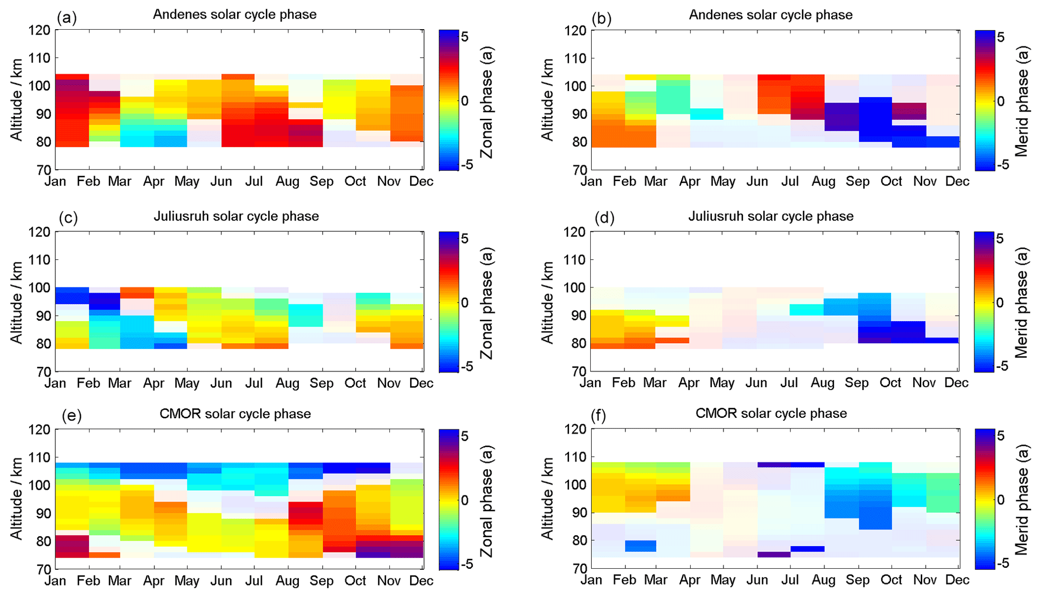
https://www.ann-geophys.net/37/851/2019/angeo-37-851-2019-f21

Figure A1Phase information of the solar cycle fit for the wind component. The shaded areas are not significant.

Download

https://www.ann-geophys.net/37/851/2019/angeo-37-851-2019-f22

Figure A2Same as Fig. A1 but for the diurnal component.

Download

https://www.ann-geophys.net/37/851/2019/angeo-37-851-2019-f23

Figure A3Same as Fig. A1 but for the semidiurnal component.

Download

Author contributions

SW wrote the manuscript with input from all the authors. Furthermore, all the co-authors contributed to the data interpretation. GS provided the high-resolution meteor wind data analysis for all the stations and ensured the operation of the Andenes and Juliusruh meteor radar. PB ensures the operation of the CMOR meteor radar.

Competing interests

The authors declare that they have no conflict of interest.

Acknowledgements

This work was partly supported by the WATILA project (SAW-2015-IAP-1 383) and partly by the Deutsche Forschungsgemeinschaft (DFG, German Research Foundation; project no. LU1174, PACOG as part of the MS-GWaves research unit). Furthermore, we acknowledge the IAP technicians for the technical support. We are thankful for discussions with Peter Hoffmann.

Financial support

The publication of this article was funded by the Open Access Fund of the Leibniz Association.

Review statement

This paper was edited by Dalia Buresova and reviewed by two anonymous referees.

References

Baumgarten, K. and Stober, G.: On the evaluation of the phase relation between temperature and wind tides based on ground-based measurements and reanalysis data in the middle atmosphere, Ann. Geophys., 37, 581–602, https://doi.org/10.5194/angeo-37-581-2019, 2019. a

Baumgarten, K., Gerding, M., Baumgarten, G., and Lübken, F.-J.: Temporal variability of tidal and gravity waves during a record long 10-day continuous lidar sounding, Atmos. Chem. Phys., 18, 371–384, https://doi.org/10.5194/acp-18-371-2018, 2018. a, b

Becker, E.: Dynamical Control of the Middle Atmosphere, Space Sci. Rev., 168, 283–314, https://doi.org/10.1007/s11214-011-9841-5, 2012. a

Beig, G.: Long-term trends in the temperature of the mesosphere/lower thermosphere region: 1. Anthropogenic influences, J. Geophys. Res., 116, A00H11, 2011. a

Brown, P., Weryk, R., Wong, D., and Jones, J.: A meteoroid stream survey using the Canadian Meteor Orbit Radar: I. Methodology and radiant catalogue, Icarus, 195, 317–339, https://doi.org/10.1016/j.icarus.2007.12.002, 2008. a

Chau, J. L., Hoffmann, P., Pedatella, N. M., Matthias, V., and Stober, G.: Upper mesospheric lunar tides over middle and high latitudes during sudden stratospheric warming events, J. Geophys. Res.-Space Phy., 120, 3084–3096, https://doi.org/10.1002/2015JA020998, 2015. a

Conte, J. F., Chau, J. L., Stober, G., Pedatella, N., Maute, A., Hoffmann, P., Janches, D., Fritts, D., and Murphy, D. J.: Climatology of semidiurnal lunar and solar tides at middle and high latitudes: Interhemispheric comparison, J. Geophys. Res.-Space Phy., 122, 7750–7760, https://doi.org/10.1002/2017JA024396, 2017. a

Conte, J. F., Chau, J. L., Laskar, F. I., Stober, G., Schmidt, H., and Brown, P.: Semidiurnal solar tide differences between fall and spring transition times in the Northern Hemisphere, Ann. Geophys., 36, 999–1008, https://doi.org/10.5194/angeo-36-999-2018, 2018. a

Dowdy, A., Vincent, R. A., Tsutsumi, M., Igarashi, K., Murayama, Y., Singer, W., and Murphy, D. J.: Polar mesosphere and lower thermosphere dynamics: 1. Mean wind and gravity wave climatologies, J. Geophys. Res.-Atmos., 112, D17104, https://doi.org/10.1029/2006JD008126, 2007. a

Eckermann, S. D., Broutman, D., Ma, J., Doyle, J. D., Pautet, P. D., Taylor, M. J., Bossert, K., Williams, B. P., Fritts, D. C., and Smith, R. B.: Dynamics of Orographic Gravity Waves Observed in the Mesosphere over the Auckland Islands during the Deep Propagation Gravity Wave Experiment (DEEPWAVE), J. Atmos. Sci., 73, 3855–3876, https://doi.org/10.1175/JAS-D-16-0059.1, 2016. a

Egito, F., Andrioli, V., and Batista, P.: Vertical winds and momentum fluxes due to equatorial planetary scale waves using all-sky meteor radar over Brazilian region, J. Atmos. Solar-Terr. Phy., 149, 108–119, https://doi.org/10.1016/j.jastp.2016.10.005, 2016. a

Emmert, J. T., Picone, J. M., and Meier, R. R.: Thermospheric global average density trends, 1967–2007, derived from oorbit of 5000 near-Earth objects, Geophys. Res. Lett., 35, L05101, https://doi.org/10.1029/2007GL032809, 2008. a

Fritts, D. C. and Alexander, M. J.: Gravity wave dynamics and effects in the middle atmosphere, Rev. Geophys., 41, 1003, https://doi.org/10.1029/2001RG000106, 2003. a, b

Fritts, D. C. and VanZandt, T. E.: Spectral Estimates of Gravity Wave Energy and Momentum Fluxes. Part I: Energy Dissipation, Acceleration, and Constraint., J. Atmos. Sci., 50, 3685–3694, https://doi.org/10.1175/1520-0469(1993)050<3685:SEOGWE>2.0.CO;2, 1993. a

Fuller-Rowell, T. J., Fang, T.-W., Wang, H., Matthias, V., Hoffmann, P., Hocke, K., and Studer, S.: Impact of Migrating Tides on Electrodynamics During the January 2009 Sudden Stratospheric Warming, chap. 14, pp. 163–174, American Geophysical Union (AGU), https://doi.org/10.1002/9781118929216.ch14, 2016. a

Geißler, C. and Jacobi, C.: Mesospheric wind and temperature trends simulated with MUAM, Meteorologische Arbeiten aus Leipzig, 22, ISBN 978-3-9814401-3-3, 2017. a, b

Hagan, M. E. and Forbes, J. M.: Migrating and nonmigrating diurnal tides in the middle and upper Atmosphere excited by tropospheric latent heat release, J. Geophys. Res., 107, 4754, https://doi.org/10.1029/2001JD001236, 2002. a

Hocking, W. K., Fuller, B., and Vandepeer, B.: Realtime determination of meteor-related parameters utilizing modern digital technology, J. Atmos. Solar-Terr. Phy., 69, 155–169, https://doi.org/10.1016/S1364-6826(00)00138-3, 2001. a

Hoffmann, P., Becker, E., Singer, W., and Placke, M.: Seasonal variation of mesospheric waves at northern middle and high latitudes, J. Atmos. Solar-Terr. Phy., 72, 1068–1079, https://doi.org/10.1016/j.jastp.2010.07.002, 2010. a, b

Hoffmann, P., Rapp, M., Singer, W., and Keuer, D.: Trends of mesospheric gravity waves at northern middle latitudes during summer, J. Geophys. Res., 116, D00P08, https://doi.org/10.1029/2011JD015717, 2011. a, b, c

Hysell, D., Fritts, D., Laughman, B., and Chau, J. L.: Gravity Wave-Induced Ionospheric Irregularities in the Postsunset Equatorial Valley Region, J. Geophys. Res., 122, 579–590, https://doi.org/10.1002/2017JA024514, 2017. a

Iimura, H., Fritts, D. C., Tsutsumi, M., Nakamura, T., Hoffmann, P., and Singer, W.: Long-term observations of the wind field in the Antarctic and Arctic mesosphere and lower-thermosphere at conjugate latitudes, J. Geophys. Res., 116, D20112, https://doi.org/10.1029/2011JD016003, 2011. a, b

Iimura, H., Fritts, D. C., Janches, D., Singer, W., and Mitchell, N. J.: Interhemispheric structure and variability of the 5-day planetary wave from meteor radar wind measurements, Ann. Geophys., 33, 1349–1359, https://doi.org/10.5194/angeo-33-1349-2015, 2015. a

Jacobi, C.: 6 year mean prevailing winds and tides measured by VHF meteor radar over Collm (51.3^∘ N, 13.0^∘ E), J. Atmos. Solar-Terr. Phy., 78–79, 8–18, https://doi.org/10.1016/j.jastp.2011.04.010, 2012. a, b, c, d, e

Jacobi, Ch., Hoffmann, P., and Kürschner, D.: Trends in MLT region winds and planetary waves, Collm (52^∘ N, 15^∘ E), Ann. Geophys., 26, 1221–1232, https://doi.org/10.5194/angeo-26-1221-2008, 2008. a

Jacobi, C., Fröhlich, K., Portnyagin, Y., Merzlyakov, E., Solovjova, T., Makarov, N., Rees, D., Fahrutdinova, A., Guryanov, V., Fedorov, D., Korotyshkin, D., Forbes, J., Pogoreltsev, A., and Kürschner, D.: Semi-empirical model of middle atmosphere wind from the ground to the lower thermosphere, Adv. Space Res., 43, 239–246, 2009. a

Jacobi, C., Lilienthal, F., Geißler, C., and Krug, A.: Long-term variability of mid-latitude mesosphere-lower thermosphere winds over Collm (51 N, 13 E), J. Atmos. Solar-Terr. Phy., 136, 174–186, https://doi.org/10.1016/j.jastp.2015.05.006, 2015. a, b, c

Jones, J., Brown, P., Ellis, K., Webster, A., Campbell-Brown, M., Krzemenski, Z., and Weryk, R.: The Canadian Meteor Orbit Radar: system overview and preliminary results, Planet. Space Sci., 53, 413–421, https://doi.org/10.1016/j.pss.2004.11.002, 2005. a

Keuer, D., Hoffmann, P., Singer, W., and Bremer, J.: Long-term variations of the mesospheric wind field at mid-latitudes, Ann. Geophys., 25, 1779–1790, https://doi.org/10.5194/angeo-25-1779-2007, 2007. a, b, c

Kishore Kumar, G. and Hocking, W. K.: Climatology of northern polar latitude MLT dynamics: mean winds and tides, Ann. Geophys., 28, 1859–1876, https://doi.org/10.5194/angeo-28-1859-2010, 2010. a

Las̆tovic̆ka, J., Solomon, S. C., and Qian, L.: Trends in the Neutral and Ionized Upper Atmosphere, Space Sci. Rev., 168, 113–145, https://doi.org/10.1007/s11214-011-9799-3, 2012. a

Latteck, R., Singer, W., Morris, R. J., Hocking, W. K., Murphy, D. J., Holdsworth, D. A., and Swarnalingam, N.: Similarities and differences in polar mesosphere summer echoes observed in the Arctic and Antarctica, Ann. Geophys., 26, 2795–2806, https://doi.org/10.5194/angeo-26-2795-2008, 2008. a

Lieberman, R. S. and Hays, P. B.: An estimate of the momentum deposition in the lower thermosphere by the observed diurnal tide., J. Atmos. Sci., 51, 3094–3105, https://doi.org/10.1175/1520-0469(1994)051<3094:AEOTMD>2.0.CO;2, 1994. a

Lindzen, R. S. and Chapman, S.: Atmospheric tides, Space Sci. Rev., 10, 3–188, https://doi.org/10.1007/BF00171584, 1969. a

Lu, H., Gray, L. J., White, I. P., and Bracegirdle, T. J.: Stratospheric Response to the 11-Yr Solar Cycle: Breaking Planetary Waves, Internal Reflection, and Resonance, J. Climate, 30, 7169–7190, https://doi.org/10.1175/JCLI-D-17-0023.1, 2017. a

Lukianova, R., Kozlovsky, A., and Lester, M.: Climatology and inter-annual variability of the polar mesospheric winds inferred from meteor radar observations over Sodankylä (67 N, 23 E) during solar cycle 24, J. Atmos. Solar-Terr. Phy., 171, 241–249, https://doi.org/10.1016/j.jastp.2017.06.005, 2018. a

Manson, A. H., Meek, C. E., Chshyolkova, T., Xu, X., Aso, T., Drummond, J. R., Hall, C. M., Hocking, W. K., Jacobi, Ch., Tsutsumi, M., and Ward, W. E.: Arctic tidal characteristics at Eureka (80^∘ N, 86^∘ W) and Svalbard (78^∘ N, 16^∘ E) for 2006/07: seasonal and longitudinal variations, migrating and non-migrating tides, Ann. Geophys., 27, 1153–1173, https://doi.org/10.5194/angeo-27-1153-2009, 2009. a

Matsuno, T.: A Dynamical Model of the Stratospheric Sudden Warming, J. Atmos. Sci., 28, 1479–1494, https://doi.org/10.1175/1520-0469(1971)028<1479:ADMOTS>2.0.CO;2, 1971. a, b

Matthias, V. and Ern, M.: On the origin of the mesospheric quasi-stationary planetary waves in the unusual Arctic winter 2015/2016, Atmos. Chem. Phys., 18, 4803–4815, https://doi.org/10.5194/acp-18-4803-2018, 2018. a, b

Middleton, H. R., Mitchell, N. J., and Muller, H. G.: Mean winds of the mesosphere and lower thermosphere at 52^∘ N in the period 1988–2000, Ann. Geophys., 20, 81–91, https://doi.org/10.5194/angeo-20-81-2002, 2002. a, b

Pedatella, N., Liu, H.-L., and Hagan, M.: Day-to-day migrating and nonmigrating tidal variability due to the six-day planetary wave, J. Geophys. Res., 117, A06301, https://doi.org/10.1029/2012JA017581, 2012. a

Pokhotelov, D., Becker, E., Stober, G., and Chau, J. L.: Seasonal variability of atmospheric tides in the mesosphere and lower thermosphere: meteor radar data and simulations, Ann. Geophys., 36, 825–830, https://doi.org/10.5194/angeo-36-825-2018, 2018. a, b, c, d, e

Portnyagin, Y. I., Solovjova, T. V., Makarov, N. A., Merzlyakov, E. G., Manson, A. H., Meek, C. E., Hocking, W., Mitchell, N., Pancheva, D., Hoffmann, P., Singer, W., Murayama, Y., Igarashi, K., Forbes, J. M., Palo, S., Hall, C., and Nozawa, S.: Monthly mean climatology of the prevailing winds and tides in the Arctic mesosphere/lower thermosphere, Ann. Geophys., 22, 3395–3410, https://doi.org/10.5194/angeo-22-3395-2004, 2004. a, b, c, d

Portnyagin, Y. I., Merzlyakov, E. G., Solovjova, T. V., Jacobi, C., Kürschner, D., Manson, A., and Meek, C.: Long-term trends and year-to-year variability of mid-latitude mesosphere/lower thermosphere winds, J. Atmos. Solar-Terr. Phy., 68, 1890–1901, https://doi.org/10.1016/j.jastp.2006.04.004, 2006. a

Qian, L., Jacobi, C., and McInerney, J.: Trends and Solar Irradiance Effects in the Mesosphere, J. Geophys. Res., 124, 1343–1360, https://doi.org/10.1029/2018JA026367, 2019. a

Rind, D., Lean, J., Lerner, J., Lonergan, P., and Leboissitier, A.: Exploring the stratospheric/tropospheric response to solar forcing, J. Geophys. Res., 113, D24103, https://doi.org/10.1029/2008JD010114, 2008. a

Salby, M. L. and Callaghan, P. F.: Influence of the Solar cycle on the Gerneral circulation of the Stratosphere and Upper Troposphere, Space Sci. Rev., 124, 287–303, https://doi.org/10.1007/s11214-006-9064-3, 2006. a

Schminder, R. and Kürschner, D.: Permanent monitoring of the upper mesosphere and lower thermosphere wind fields (prevailing and semidiurnal tidal components) obtained from LF D1 measurements in 1991 at the Collm Geophysical Observatory, J. Atmos. Terr. Phys., 56, 1263–1269, https://doi.org/10.1016/0021-9169(94)90064-7, 1994. a

Shibuya, R., Sato, K., Tsutsumi, M., Sato, T., Tomikawa, Y., Nishimura, K., and Kohma, M.: Quasi-12 h inertia–gravity waves in the lower mesosphere observed by the PANSY radar at Syowa Station (39.6^∘ E, 69.0^∘ S), Atmos. Chem. Phys., 17, 6455–6476, https://doi.org/10.5194/acp-17-6455-2017, 2017. a

Stober, G. and Chau, J. L.: A multistatic and multifrequency novel approach for specular meteor radars to improve wind measurements in the MLT region, Radio Sci., 50, 431–442, https://doi.org/10.1002/2014RS005591, 2015. a

Stober, G., Jacobi, C., and Keuer, D.: Distortion of meteor count rates due to cosmic radio noise and atmospheric particularities, Adv. Radio Sci., 8, 237–241, https://doi.org/10.5194/ars-8-237-2010, 2010. a

Stober, G., Jacobi, C., Matthias, V., Hoffmann, P., and Gerding, M.: Neutral air density variations during strong planetary wave activity in the mesopause region derived from meteor radar observations, J. Atmos. Solar-Terr. Phy., 74, 55–63, https://doi.org/10.1016/j.jastp.2011.10.007, 2012. a

Stober, G., Matthias, V., Brown, P., and Chau, J. L.: Neutral density variation from specularmeteor echo observations spanning one solar cycle, Geophys. Res. Lett., 41, 6919–6925, https://doi.org/10.1002/2014GL061273, 2014. a

Stober, G., Matthias, V., Jacobi, C., Wilhelm, S., Höffner, J., and Chau, J. L.: Exceptionally strong summer-like zonal wind reversal in the upper mesosphere during winter 2015/16, Ann. Geophys., 35, 711–720, https://doi.org/10.5194/angeo-35-711-2017, 2017. a, b, c, d

Stober, G., Chau, J. L., Vierinen, J., Jacobi, C., and Wilhelm, S.: Retrieving horizontally resolved wind fields using multi-static meteor radar observations, Atmos. Meas. Tech., 11, 4891–4907, https://doi.org/10.5194/amt-11-4891-2018, 2018. a, b, c

Tsuda, T.: Characteristics of atmospheric gravity waves observed using the MU (Middle and Upper atmosphere) radar and GPS (Global Positioning System) radio occultation, P. Jpn. Acad., B-Phys., 90, 12–27, https://doi.org/10.2183/pjab.90.12, 2014. a

Tsuda, T., Kato, S., and Vincent, R.: Long period wind oscillations observed by the Kyoto meteor radar and comparison of the quasi-2-day wave with Adelaide HF radar observations, J. Atmos. Terr. Phys., 50, 225–230, https://doi.org/10.1016/0021-9169(88)90071-2, 1988. a

Tsuda, T., Nishida, M., Rocken, C., and Ware, R. H.: A Global Morphology of Gravity Wave Activity in the Stratosphere Revealed by the GPS Occultation Data (GPS/MET), J. Geophys. Res., 105, 7257–7273, https://doi.org/10.1029/1999JD901005, 2000. a

Webster, A. R., Brown, P. G., Jones, J., Ellis, K. J., and Campbell-Brown, M.: Canadian Meteor Orbit Radar (CMOR), Atmos. Chem. Phys., 4, 679–684, https://doi.org/10.5194/acp-4-679-2004, 2004. a

Yiğit, E. and Medvedev, A.: Internal wave coupling processes in Earth’s atmosphere, Adv. Space Res., 55, 983–1003, https://doi.org/10.1016/j.asr.2014.11.020, 2015. a

Yiğit, E. K. K. P., Georgieva, K., and Ward, W.: A review of vertical coupling in the Atmosphere–Ionosphere system: Effects of waves, sudden stratospheric warmings, space weather, and of solar activity, J. Atmos. Solar-Terr. Phy., 141, 1–12, https://doi.org/10.1016/j.jastp.2016.02.011, 2016. a

Yuan, T., Schmidt, H., She, C. Y., Krueger, D. A., and Reising, S.: Seasonal variations of semidiurnal tidal perturbations in mesopause region temperature and zonal and meridional winds above Fort Collins, Colorado (40.6^∘ N, 105.1^∘ W), J. Geophys. Res., 113, D20103, https://doi.org/10.1029/2007JD009687, 2008a. a, b

Yuan, T., She, C.-Y., Krueger, D. A., Sassi, F., Garcia, R., Roble, R. G., Liu, H.-L., and Schmidt, H.: Climatology of mesopause region temperature, zonal wind, and meridional wind over Fort Collins, Colorado (41^∘ N, 105^∘ W), and comparison with model simulations, J. Geophys. Res., 113, D03105, https://doi.org/10.1029/2007JD008697, 2008b. a

Articles

Short summary

We report on long-term observations of atmospheric parameters in the mesosphere and lower thermosphere made over the last 2 decades for the northern-latitude locations of Andenes, Juliusruh, and Tavistock. The observations are based on meteor wind measurements and further include the long-term variability of winds, tides, and the kinetic energy of gravity waves and planetary waves. Furthermore, the influence on an 11-year oscillation on the winds and tides is presented.