2.1 Vlasiator

This study relies on numerical simulations using Vlasiator, a global hybrid-Vlasov model of the near-Earth plasma environment (von Alfthan et al., 2014; Palmroth et al., 2018). In the hybrid-Vlasov approach, protons are described as velocity distribution functions (VDFs) in a grid of the phase space (ordinary space and velocity space), whereas electrons are treated as a massless, charge-neutralising fluid. The time evolution of the VDFs is obtained by solving the Vlasov equation and closure of the system is achieved with Ohm's law including the Hall term (Palmroth et al., 2018).

The simulation run used in this study is a 2D–3V (two-dimensional in ordinary space and three-dimensional in velocity space) simulation in the noon–midnight meridional plane of the magnetosphere, i.e. xz in the geocentric solar magnetospheric (GSM) coordinate system. The origin of the simulation domain is set in the Earth's centre. The simulation box in ordinary space spans from $x=-\mathrm{94}{R}_{\mathrm{E}}$ (Earth radii; 1R_E=6371 km) on the nightside to $x=+\mathrm{47}{R}_{\mathrm{E}}$ on the dayside and is comprised between boundaries at $z=\pm \mathrm{57}{R}_{\mathrm{E}}$ in the north–south direction, with a grid resolution of 300 km. The inner boundary of the magnetospheric domain lies at ∼4.7R_E from the centre of the Earth. In each cell of the ordinary space, a velocity grid extends between −4020 km s⁻¹ and 4020 km s⁻¹ with a resolution of 30 km s⁻¹ in V_x, V_y and V_z. A sparsity threshold is implemented in Vlasiator, below which phase-space density values are discarded to limit the computational load of the simulation. In the run used in this study, the sparsity threshold is set to 10⁻¹⁵ m⁻⁶ s³.

The near-Earth environment is driven by incoming solar wind from the +x wall of the simulation domain. The solar wind population consists of protons characterised by Maxwellian VDFs with a number density of 1 cm⁻³, a temperature of 500 kK, a bulk velocity of −750 km s⁻¹ along the x axis and a dynamic pressure of about 0.9 nPa, carrying a purely southward IMF with a magnitude of 5 nT. Other boundary conditions are as follows: the von Neumann condition for the −x and ±z walls and periodic conditions in the out-of-plane direction (±y), and the inner boundary is a perfectly conducting cylinder with a static Maxwellian VDF for protons. Finally, the geomagnetic field is given by a 2-D line dipole along the z axis, centred at the origin and scaled to obtain a realistic magnetopause stand-off distance (Daldorff et al., 2014).

In the solar wind, the ion inertial length is λ_p=228 km, and the proton Larmor radius is r_L=214 km. A dedicated study by Pfau-Kempf et al. (2018) showed that the ordinary space resolution of 300 km is enough to resolve most of the proton kinetics in such conditions. Besides this, the Alfvén speed is V_A=109 km s⁻¹, which is significantly greater than the velocity space resolution of 30 km s⁻¹. Similarly, the ordinary space and velocity space resolutions are enough to resolve the ion kinetics in the transition region between stretched and dipole-like magnetic field lines in the magnetotail, where λ_p=906 km, r_L=681 km and V_A=1596 km s⁻¹.

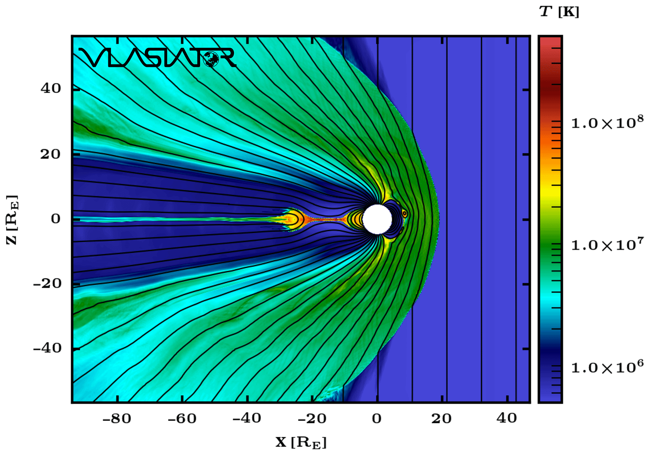
Figure 1Simulated plasma temperature in the entire simulation domain at t=1800 s. The white area corresponds to near-Earth space located inside the inner boundary at 4.7 R_E. Black lines represent magnetic field lines.

Figure 1 gives an overview of the simulated area at a time step (t=1800 s) when nightside reconnection takes place. The plotted parameter is the plasma temperature, and the black lines correspond to magnetic field lines. The incoming solar wind at 500 kK with a southward IMF can be seen on the right-hand side of the figure, and the major geospace regions (bow shock, magnetosheath, dayside magnetopause, polar cusps, magnetotail lobes and plasma sheet) can be identified. A plasmoid is forming in the nightside magnetosphere (Palmroth et al., 2017), whose signature is visible between $x=-\mathrm{30}{R}_{\mathrm{E}}$ and $x=-\mathrm{20}{R}_{\mathrm{E}}$. Juusola et al. (2018b) studied the plasma sheet during this same run and evaluated its thickness to lie essentially within 0.1–0.2 R_E (i.e. just a few simulation cells) in the region of interest for our study ($x>-\mathrm{20}{R}_{\mathrm{E}}$).

This simulation run was previously used in several studies focusing on various phenomena and regions in the near-Earth space, such as dayside magnetopause reconnection (Hoilijoki et al., 2017), ion acceleration in the magnetosheath (Jarvinen et al., 2018), magnetotail reconnection (Palmroth et al., 2017; Juusola et al., 2018a) and magnetotail current-sheet flapping (Juusola et al., 2018b). In each of these studies, the presented results showed good correspondence with earlier findings. Here, this run will be used to characterise nightside auroral proton precipitation in the simulation by making use of the VDF description of the proton population.

2.2 Precipitation spectra calculation

Figure 2 illustrates the definitions of angles and vectors used in this section. The configuration is shown for particles precipitating in the Southern Hemisphere to be consistent with the results shown in the rest of the paper. For particles precipitating in the Northern Hemisphere, the configuration is symmetrical.

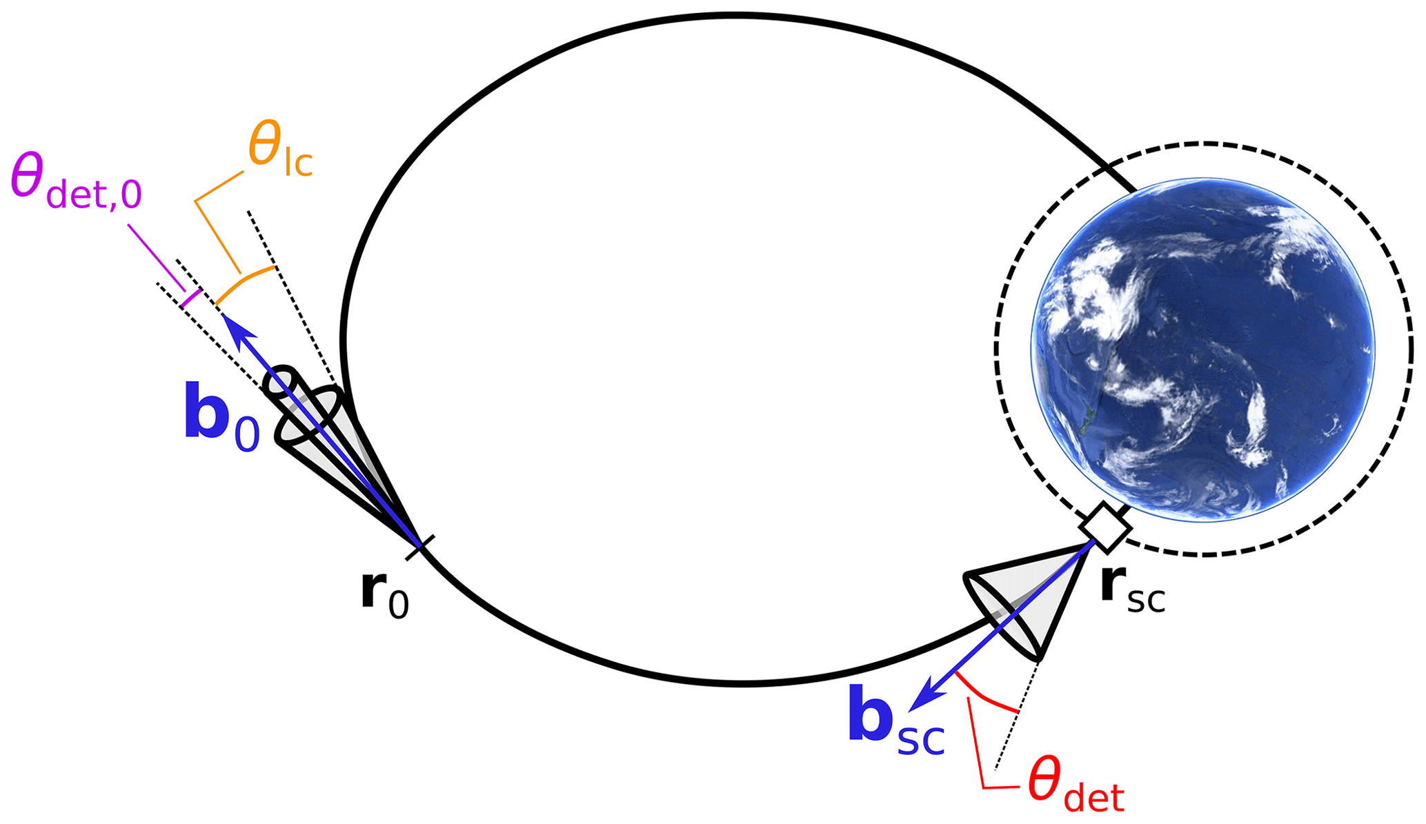
Figure 2Geometry used in the derivation of directional differential flux of precipitating protons.

At a given three-dimensional location r of the ordinary space, the differential intensity 𝒥 (more generally called directional differential flux) of protons at energy E for the direction along unit vector u is related to the velocity distribution function f by (Eq. 6.47 in Baumjohann and Treumann, 1997)

where m_p is the proton mass and $v=\sqrt{\mathrm{2}E/m_{\mathrm{p}}}$ is the velocity magnitude. 𝒥, when expressed in SI units, is given in particles per square metre per second per steradian per joule.

Particle detectors aboard spacecraft estimate 𝒥 by taking the average of the incoming particle flux in a given energy channel over the detector's surface S_det and viewing angle Ω_det, which can be written as

where u^′ is the unit vector of a given velocity direction inside Ω_det, n_det is the unit vector normal to the detector's surface and r_sc is the location of the spacecraft, for instance near the top of the ionosphere. Strictly speaking, $\widehat{\mathcal{J}}$ is a differential intensity measured within a fixed solid angle and detector area. In practice, telescopes aboard spacecraft generally collect particles within a cone with an opening angle θ_det of the order of 15^∘ (e.g. Rodger et al., 2010). Assuming that the directional differential flux is uniform over the detector's surface and that n_det is aligned with the local geomagnetic field direction b_sc (i.e. the telescope measures precipitating particles), and expressing the velocity distribution function in spherical coordinates $(v,\mathit{\theta },\mathit{\phi })$ in the local magnetic frame, one gets

or, by defining μ=cos θ,

with μ_det=cos θ_det. In the symmetrical configuration where the spacecraft observes precipitating particles in the Northern Hemisphere, n_det is aligned with −b_sc, but angle definitions remain the same.

As a first-order approximation, protons remain attached to a given magnetic flux tube; one can hence trace particles backwards in time out to the magnetosphere, following magnetic field lines. Assuming smooth quasi-linear propagation, for a given particle of pitch angle θ, the quantity sin ²θ∕B is conserved along the trajectory. Let r₀ be a location in the magnetosphere mapping to the spacecraft in terms of magnetic field topology. For particles travelling between r₀ and r_sc, we have

where B₀ and θ₀ correspond to the magnetic field magnitude and the particle pitch angle at r₀, respectively, and B_sc and θ correspond to the same parameters at r_sc. This can also be written as

with μ₀=cos θ₀. By differentiating Eq. (6), one gets

According to Liouville's theorem, $f(\mathit{r},v,\mathit{\mu },\mathit{\phi })$ is conserved along the trajectories of the system, i.e. in the absence of potential fields:

Using Eq. (8), and then Eqs. (6) and (7), yields, from Eq. (4),

where b₀ is the unit vector with the direction of the local magnetic field at r₀, and

In other words, the directional differential particle flux observed by the telescope aboard the spacecraft can be estimated by averaging the relevant subset of the particle VDF at a chosen conjugate location in the magnetosphere. The angular boundaries of the averaged phase-space domain are obtained by scaling the viewing angle of the detector to ${\mathit{\theta }}_{\det ,\mathrm{0}}=\arccos {\mathit{\mu }}_{\det ,\mathrm{0}}$ based on the ratio of magnetic field magnitudes at the spacecraft and at the conjugate location in the magnetosphere where the VDF is analysed (see Eq. 10).

For particles located at r₀ to reach a spacecraft at the top of the ionosphere at ∼800 km altitude, their pitch angles must be within the bounce loss cone, whose opening angle is determined by

In the undisturbed nightside equatorial plane, θ_lc takes values of a few degrees at most and is smaller than 1^∘ beyond 10 R_E (see, e.g. Sergeev and Tsyganenko, 1982). In the presence of a rather large dipolarisation front with, for example, $B_{\mathrm{0}}\simeq B_z=\mathrm{30}$ nT, assuming a mapping to auroral latitudes (B_sc∼53 000 nT), as in Eq. (11), gives ${\mathit{\theta }}_{\mathrm{lc}}=\mathrm{1.4}{}^{\circ }$. In Vlasiator, knowing the VDF at a given location in the magnetosphere, one can calculate the bounce loss-cone angle value and, at a given velocity magnitude v (i.e. at a given energy), average the phase-space density inside the loss cone to evaluate $\widehat{\mathcal{J}}(E,{\mathit{b}}_{\mathrm{0}},{\mathit{r}}_{\mathrm{0}})$. It should be noted that, with this approach, the obtained directional differential precipitating flux corresponds to the differential flux which would be measured by a telescope aboard a spacecraft at the topside ionosphere with a viewing angle Ω_det=2π sr (see Eq. 2).

In practice, the methodology to estimate differential precipitating proton fluxes at r₀ is as follows. First, the loss-cone angle θ_lc is calculated. This is achieved by following the magnetic field line from r₀ to the inner boundary of the simulation domain, at about 4.7 R_E, and then extrapolating the magnetic field to the top of the ionosphere using the line dipole approximation. The ratio of the magnetic field magnitudes at r₀ and at the mapped region in the topside ionosphere enables the calculation of the bounce loss-cone angle using Eq. (11). Second, we estimate the differential precipitating flux by calculating

where ${〈f({\mathit{r}}_{\mathrm{0}},v,\mathit{\theta },\mathit{\phi })〉}_{\mathit{\theta }<{\mathit{\theta }}_{\mathrm{0}}}$ is the average value of the phase-space density at speed v inside the bounce loss cone. This approximation of Eq. (9) is reasonable, since θ₀ is very small, and hence we have ${\mathit{\mu }}_{\mathrm{0}}=\cos {\mathit{\theta }}_{\mathrm{lc}}\approx \mathrm{1}$ inside the integral.

Figure 3(a) Simulated plasma temperature in the nightside magnetosphere at t=1800 s. The Sun is located beyond the right boundary of the figure. The two black circles filled with white are virtual spacecraft S₁ and S₂. The arrows indicate the magnetic field directions at S₁ and S₂. (b) Velocity distribution function of protons at S₁ in the (v_B, v_B×V) plane. The grid spacing is 1000 km s⁻¹. The magenta lines indicate the boundaries of the bounce loss cone. (c) Same for protons at S₂.

Download

2.3 Examples of differential precipitating proton fluxes with Vlasiator

In the simulation used in this study, full velocity distributions of protons are saved every 50 simulation cells in the x and z directions due to limitations in the file sizes. Therefore, the estimation of the differential precipitating proton flux based on Eq. (12) can be applied only in a few selected locations in the nightside magnetosphere. Figure 3 shows examples of velocity distributions observed at two virtual spacecraft S₁ and S₂ that are used in this study. Figure 3a shows the proton temperature in the nightside part of the noon–midnight plane at time step t=1800 s, with magnetic field lines drawn in black. It should be stressed that this temperature is that of the isotropic plasma which would have the same total pressure as the simulated distribution; thus it does not represent the temperature of the bulk plasma but rather the measured effect of combined bulk plasma and potential fast additional flows. The effect of such a combination can be seen near S₁, as a stream of hot (T≈20 MK) plasma coming from the transition region reaches the virtual spacecraft, leading to a local enhancement of the proton temperature compared to its background value at S₁. The white area corresponds to the region of the geospace located earthwards from the inner boundary at ∼4.7R_E. Black arrows indicate the magnetic field direction at the virtual spacecraft. Figure 3b and c show slices of the velocity distributions at S₁ and S₂, respectively, in the plane defined by the local magnetic field direction v_B and the local electric field direction v_B×V (approximately aligned with the y direction, i.e. into the simulation plane). The grid spacing is 1000 km s⁻¹. The velocity distribution at S₁ consists of a core population centred near the origin and a crescent-shaped beam at about 1000 km s⁻¹. It corresponds to the superposition of cold plasma with a low bulk velocity in the magnetic field direction with a more energetic population travelling earthwards. The velocity distribution at S₂ is nearly Maxwellian, with a broad loss cone in the magnetic field direction (this loss cone will be discussed below). The width of the distribution, centred near the origin, indicates that it corresponds to hotter plasma (in comparison with the one at S₁) nearly at rest in the local magnetic frame, with protons having velocities up to about 2000 km s⁻¹. The imposed static Maxwellian VDF at the inner boundary can affect the neighbouring cells through the calculation of translation and acceleration terms in the Vlasov equation, but such effects vanish rapidly with distance to the boundary, and the plasma at S₂ is unlikely to be affected by the boundary condition.

The contrast between the velocity distributions at S₁ and S₂ is reflected in the plasma temperature, which is 15 MK at S₁ and 32 MK at S₂. In Fig. 3b and c, the bounce loss cone is indicated with pink lines. As can be seen in the two examples, the loss cone is not empty, and hence a directional differential flux of precipitating protons can be derived using Eq. (12). We note that the empty part of the phase space in Fig. 3c is due to the presence of the inner boundary. Indeed, the inner boundary absorbs incoming protons, and particles bouncing back from a mirror point earthwards from the inner boundary in the Southern Hemisphere are therefore absent at virtual spacecraft S₂ in the simulation. This feature does not have consequences in our study, since the relevant part of the velocity distribution function is the one located inside the bounce loss cone.

Figure 4(a, b, c, d) Examples of proton velocity distribution slices in the local magnetic frame at virtual spacecraft S₁ and S₂ at various time steps of the simulation. The bounce loss cone is shown with magenta lines. (e, f, g, h) Corresponding directional differential precipitating fluxes obtained with the presented method.

Download

Figure 4 shows four examples of velocity distributions at virtual spacecraft S₁ and S₂ during the simulation run (Fig. 4a–d) and the associated precipitating proton differential fluxes obtained using the method described in Sect. 2.2 (Fig. 4e–h). The velocity distributions are slices in the plane defined by the magnetic field direction, v_B, and the electric field direction, v_B×V. Figure 4a and b are the distributions at t=1800.0 s at virtual spacecraft S₁ and S₂, respectively, shown in Fig. 3. The crescent-shaped beam partly in the bounce loss cone shown in Fig. 4a is associated with a precipitating differential flux narrow in energies (Fig. 4e), peaking at around 4–5 keV with values close to 10⁴ proton cm⁻² s⁻¹ sr⁻¹ eV⁻¹. Although this distribution is intrinsically unstable, the development of instabilities (magnetosonic, ion–ion left-hand and firehose) requires the conditions that the field-aligned drift velocity V₀ of the protons be greater than the Alfvén speed V_A and that the ratio between beam (n_b) and core (n_c) densities be “very small” (Gary, 1991). While the distribution shown in Fig. 4a has $n_{\mathrm{b}}/n_{\mathrm{c}}=\mathrm{0.086}$, it exhibits V₀∼1000 and V_A=4379 km s⁻¹. Since the criterion on velocities is not verified, we do not expect that the instabilities listed above can grow fast enough to significantly affect the ion distributions on the timescale needed for precipitating protons (i.e. essentially the field-aligned beam) to reach the inner boundary or even the ionosphere.

In contrast with the distribution with a crescent-shaped beam shown in Fig. 4a, the hot, nearly Maxwellian velocity distribution inside the loss cone at S₂ (Fig. 4b) is associated to a broad precipitation spectrum (Fig. 4f), with energies of precipitating protons ranging from below 100 eV to nearly 30 keV. The peak differential flux values are of the order of 4000 proton cm⁻² s⁻¹ sr⁻¹ eV⁻¹, at energies of 2–5 keV. The sharp cut-off taking place at ∼25 keV in Fig. 4f is due to the sparsity threshold, set to 10⁻¹⁵ m⁻⁶ s³ in this run, hence corresponding to the lower limit of the colour axis in Fig. 4a–d. Figure 4c shows a velocity distribution relatively similar to Fig. 4a but was obtained at virtual spacecraft S₂ with a delay of 100 s, indicating that the region with narrow-beam precipitation moved earthwards. The corresponding differential flux in Fig. 4g is centred around 2–3 keV, i.e. slightly lower than in Fig. 4e, while peak flux values are almost the same, with nearly 10⁴ proton cm⁻² s⁻¹ sr⁻¹ eV⁻¹. The last velocity distribution, in Fig. 4d, was taken at S₁ 200 s after the one from Fig. 4a. The core population is broader and is partly inside the bounce loss cone, leading to a low flux of low-energy (0.1–1 keV) proton precipitation, as can be seen in Fig. 4h. A beam of low phase-space density with a complex structure partly fills the loss cone at velocities of 1300–2100 km s⁻¹, which is shown in the precipitating spectrum as two peaks, at about 8 and 15 keV, with flux values 2 orders of magnitude lower than in Fig. 4a. These four selected examples suggest that at virtual spacecraft S₁ and S₂, one can observe a variety of precipitating fluxes during the Vlasiator simulation. If compared to observations, these differential fluxes are within the same order of magnitude as the NOAA 6 proton energy spectra shown in Basu et al. (2001) in terms of peak energy (1–10 keV) and slightly higher in terms of flux values (10²–10³ cm⁻² s⁻¹ sr⁻¹ eV⁻¹). Observations from the DMSP 12 spacecraft reported in Lummerzheim et al. (2001) indicate mean precipitating energy of the order of 10 keV and flux values around 10³ cm⁻² s⁻¹ sr⁻¹ eV⁻¹. These values were, however, obtained in the evening MLT sector, where proton precipitation exhibits statistically harder energy spectra than in the midnight sector (Galand et al., 2001).

One assumption which is made during the derivation of the precipitating fluxes is that there are no field-aligned electric fields in the system (see Eq. 8). Figure S1 in the Supplement shows the parallel component of the electric field at the same time step and with a similar format to Fig. 3. This parallel component was averaged over 120 s, which corresponds roughly to one bounce period for 10 keV protons at L=9 (virtual spacecraft S₁). It can be seen that the parallel electric field between S₁ or S₂ and the inner boundary is of the order of 0.01 to 0.1 mV m⁻¹. When integrated along the field line between S₁ and the inner boundary, this corresponds to a potential difference of the order of 1 kV. In their discussion of the effect of potential drops in the auroral acceleration region on precipitating protons, Liang et al. (2013) estimate that for ions with energies ≫1 keV the acceleration resulting from typical potential drops in the auroral acceleration region (∼1 kV up to ∼4 kV occasionally) can be neglected, which enables a reasonable mapping of auroral latitudes to the central plasma sheet. It therefore seems acceptable to neglect the effect of parallel electric fields when deriving the precipitating proton fluxes with the method described in Sect. 2.2. Furthermore, given the location of S₁ and S₂ on closed field lines which are being convected earthwards, there is no risk that the precipitating protons observed at S₁ (or S₂) are affected by processes such as magnetic reconnection before they reach the ionosphere.

3.1 Nightside proton precipitation

An overview of the dynamics of the nightside magnetosphere from t=1000 s until the end of the simulation at t=2150 s is provided with Animation S1 in the Supplement. Figure 5 shows the time evolution of the proton precipitation at virtual spacecraft S₁ and S₂ during this time interval. Figure 5a and b show the precipitating proton differential flux (colour scale) as well as the mean precipitating energy (black line) as a function of time, while Fig. 5c and d show the integral energy flux. It can be seen that, at virtual spacecraft S₁, broad-energy proton precipitation above 1 keV starts at around t=1360 s, as the magnetic field line observed by S₁ becomes slightly stretched. The energetic tail of the proton precipitation spectrum reaches up to 20 keV, and the mean precipitating energy fluctuates between 2 and 5 keV until t≈1750 s, i.e. about 90 s after the global magnetotail reconfiguration is initiated by the dominant X line near $x=-\mathrm{13}{R}_{\mathrm{E}}$. At around t=1750 s, the precipitation becomes narrower in energy, and after t=1850 s, the mean precipitating energy increases from 4 to 20 keV, while fluxes decrease by almost 2 orders of magnitude. This corresponds to the times during which the nightside reconnection speeds up and S₁ observes magnetic field lines becoming more dipolar. Between t=1900 and t=1925 s, S₁ does not observe any precipitation, as the virtual spacecraft is momentarily observing lobe-type plasma and the local loss cone is empty, but precipitation resumes with high energy (10–20 keV) and relatively low differential flux values (∼10² cm⁻² s⁻¹ sr⁻¹ eV⁻¹) after t=1925 s, as S₁ is magnetically connected to the transition region. A low-energy (<1 keV) precipitating population appears between t=1990 and t=2040 s, presumably associated with heating of the core plasma. At the end of the simulation, the precipitating mean energy decreases while differential flux values are enhanced to ∼10³ cm⁻² s⁻¹ sr⁻¹ eV⁻¹. The integral energy flux remains within 1–6×10⁷ keV cm⁻² s⁻¹ sr⁻¹ during the broad-energy precipitation phase but then drops between 10⁶ and 10⁷ keV cm⁻² s⁻¹ sr⁻¹ during the phase when field lines passing by S₁ become dipolar (t=1800–1900 s). When precipitation observations from S₁ resume (t≈1930 s), the integral energy flux remains close to 10⁷ keV cm⁻² s⁻¹ sr⁻¹ before briefly increasing to reach 10⁸ keV cm⁻² s⁻¹ sr⁻¹ and abruptly decreasing around 10⁶ keV cm⁻² s⁻¹ sr⁻¹ until the end of the simulation. Those integral energy flux values are in agreement with the Hardy model, according to which the nightside maximum total energy flux ranges between about 4×10⁷ and 2×10⁸ keV cm⁻² s⁻¹ sr⁻¹, depending on the Kp index value (Hardy et al., 1989).

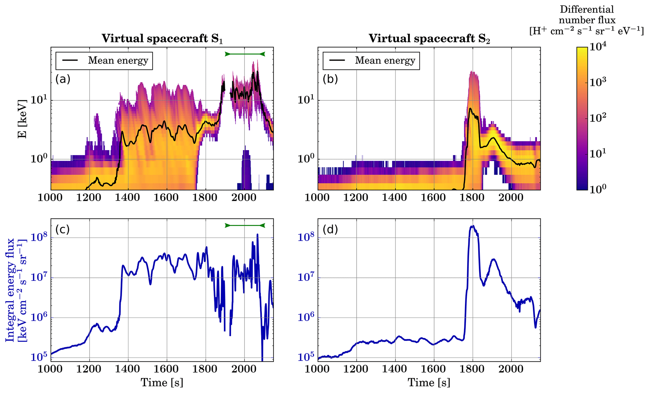
Figure 5(a) Differential number flux of precipitating protons observed at virtual spacecraft S₁ as a function of time during the simulation. The black line indicates the mean precipitating energy as a function of time. (b) Same but at virtual spacecraft S₂. (c) Integral energy flux associated with proton precipitation as a function of time at virtual spacecraft S₁.(d) Same but at virtual spacecraft S₂. The green segments in panels (a) and (c) indicate the time interval with precipitation associated with dipolarising flux bundles presented later.

Download

At virtual spacecraft S₂ (Fig. 5b and d), proton precipitation above 1 keV appears at around t=1760 s in the simulation, corresponding roughly to the time when the broad-energy precipitation at S₁ becomes narrower in energy. For about 1 min, broad-energy precipitation with up to 30 keV protons and with a mean energy of 6–7 keV is observed, leading to integral flux values reaching 2×10⁸ keV cm⁻² s⁻¹ sr⁻¹. The precipitating energy spectrum then becomes narrower and centred around 2 keV (during t=1850–1900 s) and gradually broadens again until the end of the simulation, when the mean precipitating energy decreases below 1 keV.

While the 2-D simulation set-up with a scaled line dipole does not enable a direct mapping of the virtual spacecraft locations in terms of geomagnetic latitudes or even L values, it appears clearly that the properties and the dynamics of proton precipitation are very different at S₁ and S₂. From the geometry, S₁ maps to higher geomagnetic latitudes than S₂, and the analysis of Fig. 5 suggests that S₁ represents geomagnetic latitudes which usually map to the auroral oval well, while S₂ would correspond to slightly lower latitudes where the proton auroral arc can be observed around the onset of ionospheric substorms after drifting equatorwards during the growth phase (Liu et al., 2007). Indeed, precipitation is observed at S₁ before the global magnetotail reconfiguration due to reconnection is initiated (around t=1660 s; Palmroth et al., 2017), which suggests that S₁ maps to geomagnetic latitudes where the aurora is visible during the growth phase of substorms. On the other hand, proton precipitation is only observed at S₂ around the time when the first particles that were accelerated earthwards following the global magnetotail reconfiguration reach the inner magnetosphere.

3.2 Flow bursts and precipitation

In what follows, we will focus on the proton precipitation associated with dipolarising flux bundles by considering virtual spacecraft S₁ between t=1920 and t=2080 s. During this time span, S₁ is on magnetic field lines mapping to the transition region near $x=-\mathrm{9}{R}_{\mathrm{E}}$, as can be seen in Animation S2 in the Supplement. Juusola et al. (2018a) showed that, during this time period, sustained tail reconnection takes place at a dominant X line drifting from $x\approx -\mathrm{14}$ to $x\approx -\mathrm{18}{R}_{\mathrm{E}}$ and is associated with fast earthward flows on the earthward side of the X line.

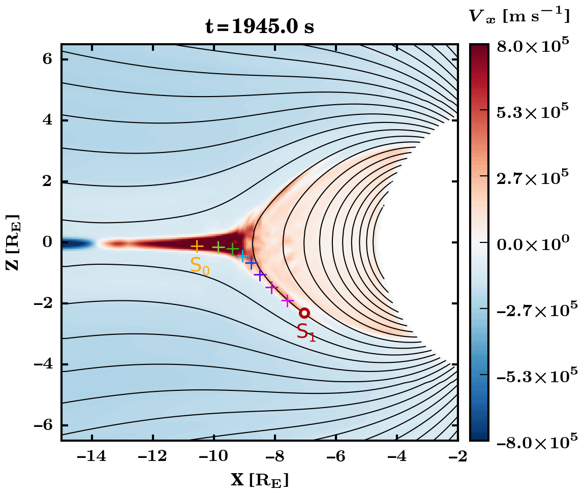
Figure 6x component of the plasma bulk velocity in the nightside part of the simulation plane at t=1945.0 s. The red circle indicates the location of virtual spacecraft S₁, and the eight coloured plus signs show additional virtual spacecraft for which the parallel velocity components are shown in Fig. 7. Black lines represent magnetic field lines.

Download

Figure 6 is a snapshot of Animation S2 at t=1945 s. The colour-coded parameter is the x component of the plasma bulk velocity, V_x. The location of virtual spacecraft S₁ is indicated with a red and white circle. Eight plus signs of various colours indicate locations of additional virtual spacecraft which will be used in the following to track the field-aligned component of the plasma bulk velocity. These virtual spacecraft are arranged in such a way that one can follow the bulk properties of the plasma between S₁ and the current sheet through the transition region. As can be seen in the figure, they are not located on a same field line but rather along the region of positive V_x, which corresponds to the path followed by precipitating protons as field lines are being convected earthwards. Full velocity distributions are not available at those points due to limitations in the file sizes. The spacecraft indicated with an orange plus sign, which is the furthest in the current sheet, will be called S₀.

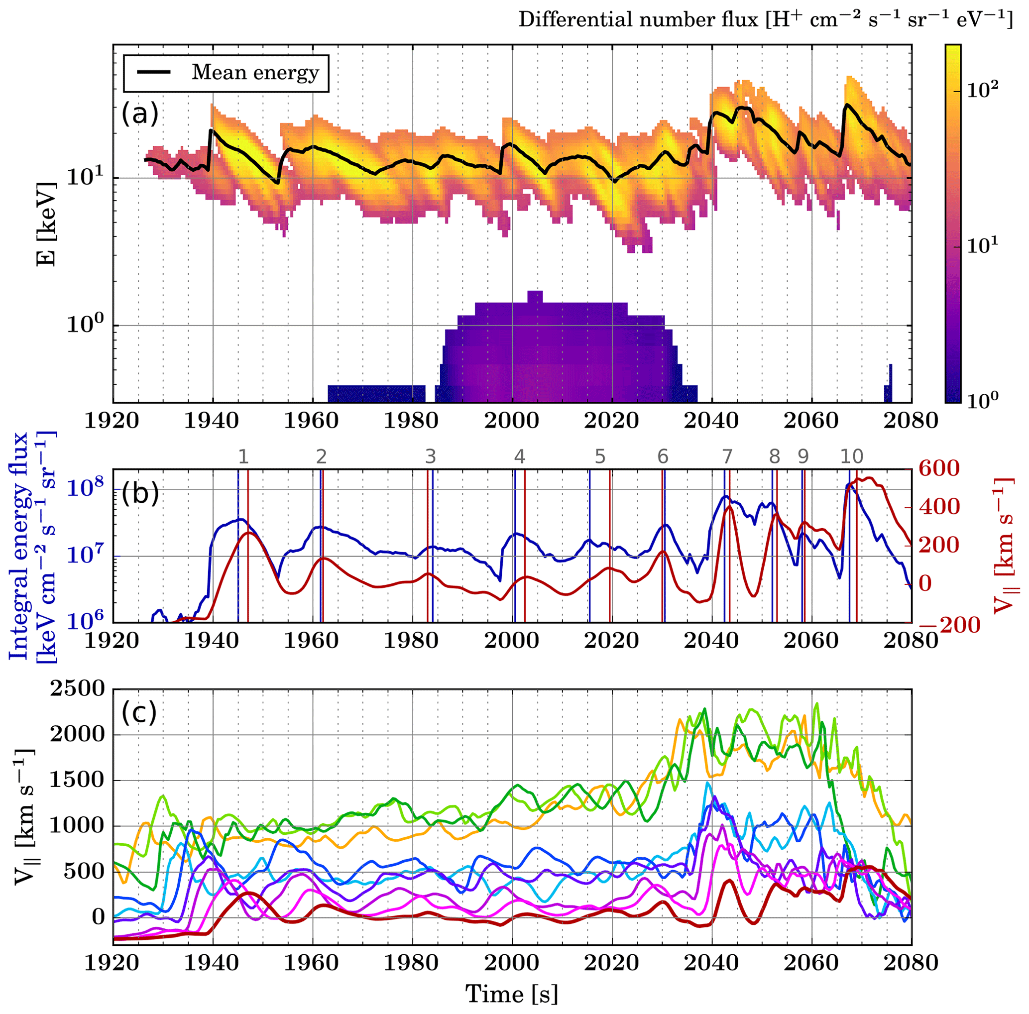
Figure 7(a) Differential number flux of precipitating protons observed at virtual spacecraft S₁ between t=1920 and t=2080 s. The black line indicates the mean precipitating energy as a function of time. (b) Blue line: integral energy flux associated with proton precipitation as a function of time at virtual spacecraft S₁. Red line: parallel component of the plasma bulk velocity at S₁. The vertical lines indicate the times associated with peak values for these two parameters, and the numbers in grey above the panel identify the precipitation bursts discussed in the text. (c) Parallel component of the plasma bulk velocity at S₁ and at the virtual spacecraft indicated with plus signs in Fig. 6, with a consistent colour code.

Download

Figure 7 shows the precipitation flux observed at S₁ between t=1920 and t=2080 s, corresponding to the time interval marked with a green line in Fig. 5a and c. Figure 7a shows the differential number flux of precipitating protons (colour scale) and the mean precipitating energy (black line). One can visually identify successive bursts of precipitating protons at energies ranging between about 5 and 50 keV. The energy dispersion of precipitating protons is visible, as within a given precipitation burst the highest energies are observed first and the lowest energies are observed last. This is also visible in the time variations of the mean precipitating energy. Between t=1985 and t=2035 s, a low-energy (<1 keV) population of precipitating protons is observed in addition to the ∼10 keV precipitation, but with fluxes lower than the main precipitating population around 10 keV by almost 2 orders of magnitude. The differential flux of the main precipitating proton population at 5–50 keV has values around 10² cm⁻² s⁻¹ sr⁻¹ eV⁻¹, which is relatively low compared to flux values at other times in the simulation that can reach 10⁴ cm⁻² s⁻¹ sr⁻¹ eV⁻¹ (see Fig. 5a). Figure 7b shows the integral energy flux (blue line) alongside the component of the plasma bulk velocity at S₁, parallel to the magnetic field (red line), V_∥. Signatures of the precipitation bursts seen in Fig. 7a can be identified in both the integral energy flux and the plasma parallel bulk velocity. This suggests that the parallel bulk velocity can be used as a proxy for precipitating protons in this context.

In Fig. 7c, the time series of the plasma parallel bulk velocity at the virtual spacecraft shown in Fig. 6 are indicated with a colour code consistent with that of the symbols indicating virtual spacecraft locations. The thick red line corresponds to the parallel velocity at S₁; i.e. it shows the same data as the red line in Fig. 7b. A given fluctuation in the parallel velocity at S₁ can be traced back in time and tailwards by visually identifying its corresponding signature at successive tailward virtual spacecraft. For instance, the parallel velocity enhancement peaking at S₁ around t=1947 s is consistent with parallel velocity enhancements visible at each of the virtual spacecraft, from the magenta one which is the closest to S₁ until the orange one (S₀), which is the deepest in the current sheet, peaking around t=1927 s. This suggests that some dipolarising flux bundles, which are identified through short-lived enhancements in $V_x\approx V_{\parallel }$ in the current sheet, directly lead to proton precipitation into the ionosphere in the regions mapped to the current sheet. However, not all the V_∥ enhancements at S₁ can be related to V_x enhancements in the current sheet. For instance, the V_∥ peak at S₁ around t=2030 s cannot be traced back to a specific V_∥ peak at S₀.

Table 1Times of peak integral energy flux and plasma bulk parallel velocities at S₁ and S₀ for the main bursts of proton precipitation. In the last column, an en dash indicates whenever a given precipitation burst observed at S₁ could not be traced back to S₀.

Download Print Version | Download XLSX

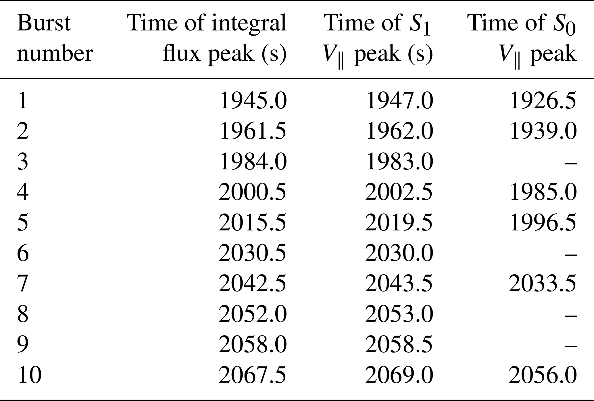
Table 1 gives the peak times of the integral energy flux, plasma bulk parallel velocity at S₁ and plasma bulk parallel velocity at S₀ for the 10 main precipitating flux enhancements between t=1920 and t=2080 s. These times correspond to those of local maxima of each parameter, as indicated with vertical lines in Fig. 7b for the integral energy flux and the parallel velocity at S₁. For the four precipitation bursts observed at S₁ which could not be traced back to S₀ in the current sheet, the time of the S₀ V_∥ peak is replaced with an en dash in the last column. In all cases but one, the peak times for the integral energy flux and V_∥ at S₁ are the same within 2 s; the exception is burst number 5, for which the triple peak in flux is associated with a single broad peak in V_∥, with a 4 s difference in the times of local maxima.

In the four cases where a precipitation burst cannot be directly linked to a DFB passing by S₀, the signatures are lost between the cyan and blue spacecraft (burst number 3), between the blue and indigo spacecraft (burst number 6), between the indigo and purple spacecraft (burst number 8), and between the light and dark green spacecraft (burst number 9). These virtual spacecraft are located in the transition region, which suggests that the transition region can act like a buffer for DFBs, either directly transmitting them and leading to bursts of precipitating protons or releasing precipitating particles with no direct correlation with an incoming DFB from the tail.