Poleward expansion of auroras arising out of the onset arc was observed in the initial pulse of Pi2 pulsations (Saka et al., 2012). Statistical study of field line inclinations at geosynchronous orbit for the intervals from 120 min prior to the Pi2 onset (T−120) to 60 min after the onset (T+60) is presented in Fig. 1 (reproduced from Saka et al., 2010). The inclination is measured positive northward from the D–V plane of the HVD coordinates. H is positive northward parallel to dipole axis, V is radial outward, and D is dipole east. It shows that field line inclination at geosynchronous orbit (Goes5/6 at 285/252^∘ in geographic coordinates) decreased continuously in the growth phase and attained minimum inclination angles, 33.6/49.4^∘, 2 min before the initial peak of Pi2 amplitudes. These inclination angles are smaller than 57.5/63.8^∘ estimated by the IGRF (International Geomagnetic Reference Field) model but rather fit the T89 model (Tsyganenko, 1989) for Kp=4 (34.2/45.0^∘). These field lines at the geosynchronous altitudes can be mapped to the auroral ionosphere at 63.4/62.7^∘ N in geomagnetic coordinates by T89 for Kp=4. Following the Pi2 onset, field line inclination turned to increase in a step-like manner at Goes5 while at Goes6, which is closer to the equatorial plane than Goes5, transient dipolarization pulses were observed. From these observations, we postulate that transient electric fields in DF triggered the ballooning instability of the stretched flux tubes at the arrival of BBFs. As a result, field lines turned back to dipole-like configurations by producing the convection surge. The convection surge may be observed by the geosynchronous satellites as the convection enhancement of the plasma sheet electrons due to local breakdown of the last open trajectories of plasma sheet electrons (Thomsen et al., 2002). The surge occurred in all-sky images coincident with the onset of bead-like rippling that leads to the breakups at the equatorward latitudes (Saka et al., 2014). In the subsequent Pi2 pulses, an auroral surge was observed in all-sky images between 66 and 74^∘ N in geomagnetic latitudes, referred to as a poleward boundary aurora surge (PBAS) (Saka et al., 2012). They propagated eastward or westward at the poleward boundary of the auroral zone and were interpreted as an auroral manifestation of flow bifurcation of BBFs. In this onset scenario, the field line dipolarization finished in the initial pulse of the Pi2 pulsations and increased field line inclination in a step-like manner or generated dipolarization pulses. The convection surge occurred once in the initial pulse of BBFs (DF) but was not repeated in the following pulses in the BBF train. This correlation suggests that auroral breakup may not repeat in the Pi2 wave packet but occurs at its initial pulse.

Figure 1Inclination angles in degrees measured positive northward from the V–D plane from 120 min prior to the Pi2 onset (T−120) and to 60 min after the Pi2 onset (T+60) reproduced from Saka et al. (2010). Magnetometer data of Goes 5/6 were represented in HVD coordinates: H is positive northward parallel to dipole axis, V is radial outward, and D is dipole east. Epoch superposition of 30 Pi2 events and mean angles calculated from them are plotted in top and in lower panels, respectively. Mean inclination angle at 2 min before the initial peak of Pi2 amplitudes (T=0) was 33.6^∘ for G5 and 49.4^∘ for G6 in dipole coordinate. Dipolarization was step-like at Goes5, while at Goes6 it was composed of dipolarization pulses. The average satellite latitudes estimated by T89 model were 10.3 and 7.9^∘ N for Goes5 and Goes6, respectively.

Download

We assume that westward electric fields associated with the convection surge were transmitted along the field lines to the auroral ionosphere by the guided poloidal mode (Radoski, 1967). The electric fields would be amplified during the projection into the ionosphere over 100 mV m⁻¹ and created an equatorward flow through E×B drift of the order of kilometers per second in the auroral ionosphere. The flows would be confined in a flow channel expanding north–south in the midnight sector. The low-latitude end of the flow channel was at the latitudes of the onset arc. The high-latitude end may not expand beyond the poleward boundary of auroral zone. Longitudinal width of the flow channel may form a streamer (e.g., Nishimura et al., 2010) and develops after the breakups in about 1 to 2 h of local time (∼1000 km along 65^∘ N) corresponding to the horizontal-scale size of plasma flow vortices associated with Pi2 (Saka et al., 2014).

In the flow channel, drift across the magnetic fields for the jth species (U_j⊥) can be written in the F region as (Kelley, 1989)

Here, E denotes westward electric fields in the flow channel and $\widehat{\mathit{B}}$ denotes a unit vector of the magnetic fields B, downward in the auroral ionosphere. Symbols k_B, T_j, q_j, and n are the Boltzmann constant, temperature of the jth species, charge of the jth species, and density of electrons (ions), respectively. The electric field of the order of 100 mV m⁻¹ exceeded the diffusion (second term) by 3 orders of magnitude in the low-temperature ionosphere. The E×B drift predominated in the F region and the diffusion term may be ignored. In the E region, drift trajectories may be written (Kelley, 1989) for electrons by

and for ions by

Here, b_i is the mobility of ions defined as Ω_i∕(Bν_in), and κ_i is defined as Ω_i∕ν_in. Symbols Ω_i and ν_in are ion gyrofrequency and ion-neutral collision frequency, respectively. $\widehat{\mathit{B}}$ denotes a unit vector of the magnetic fields B. To derive Eqs. (2) and (3), pressure gradient term (diffusion) was again ignored. In the E region (κ_i=0.1), plasma accumulation in equatorward latitudes by the imposed westward electric fields was produced by Eq. (2) for electrons and the second term in Eq. (3) for ions. Electrons smoothly moved equatorward while ions stopped in the original place because of low mobilities caused by high ion-neutral collisions. However, electron accumulation in lower latitudes increased southward electric fields and simultaneously ion drifts in the first term of Eq. (3) start. If the southward electric fields grew to exceed the westward electric fields by an order of magnitude, ion drifts in the first term of Eq. (3) and electron drifts in Eq. (2) balanced to satisfy the quasi-neutrality. This is equivalent to the generation of the Pedersen currents in the ionosphere. Thus, quasi-neutral electrostatic potential is generated in the E region, positive in poleward and negative in equatorward. The Pedersen currents would have closed to the field-aligned current (FAC), upward from the negative potential region and downward into the positive potential region to sustain the steady-state electrostatic potential in the ionosphere. Plasma drifts in the ionosphere, both in E and F regions, create a cavity in the high-latitude end of the flow channel and density pileup at the low-latitude end of the flow channel. We will focus on the density accumulation in the flow channel and discuss vertical transport of these accumulated materials. The development of the cavity in the flow channel may be the subject of another paper.

A transient compression of the ionospheric plasmas at the low-latitude edge of the flow channel would excite the ion acoustic wave in the ionosphere traveling along the field lines in the upward and downward directions from the density peak of the F region. Figure 2 shows altitude distribution of the pre-onset density profile of electrons (black) and doubled density profile caused by the accumulation in red. The electron density profile in black was plotted using the sunspot maximum condition in the nightside given in Prince Jr. and Bostick Jr. (1964). The traveling ion acoustic waves, upward and downward, are denoted by vertical arrows. Ion acoustic wave propagating downward may be eventually absorbed in the neutrals, while the upward wave may propagate along the field lines further upward. We will focus only on the upward-traveling ion acoustic wave. Electron motions produced the parallel electric fields in accordance with the Boltzmann relation (Chen, 1974),

Here, k_B is the Boltzmann constant, q is electron charge, T_e is electron temperature, and n_e is electron density (n_e=n_i). Equation (4) gives electric field strengths of the order of 0.4 and 2.0 µV m⁻¹ for T_e=1000 K and T_e=5000 K, respectively, when the e-folding distance of density dropout along the filed lines was 200 km. For ions, steady-state motions exist in the ionosphere in the altitudes where ion-neutral collision frequencies exceed ion acoustic wave frequencies. In that case, parallel motions can be written as (Kelley, 1989)

Here, b_i and D_i denote the mobility and diffusion coefficient of ions defined by $\frac{q_{\mathrm{i}}}{M_{\mathrm{i}}{\mathit{\nu }}_{\mathrm{in}}}$ and $\frac{k_{\mathrm{B}}{T}_{\mathrm{i}}}{M_{\mathrm{i}}{\mathit{\nu }}_{\mathrm{in}}}$, respectively. The symbols M_i, q_i, ν_in, and g are ion mass, electric charge of ions, ion-neutral collision frequency, and gravity, respectively. Ion-neutral collision frequencies from 400 to 1000 km in altitudes were plotted in Fig. 3 using the nighttime sunspot maximum condition in Prince Jr. and Bostick Jr. (1964). Frequencies of ion acoustic wave were calculated by substituting the wavelength of ion acoustic wave into the dispersion relation. The wavelength was assumed to be identical to initial accumulation distance along the field lines. We chose two cases of 1000 and 4000 km. Phase velocity of the ion acoustic wave of the order of 1600 m s⁻¹ for the electron temperatures of 5000 K yields the wave frequencies of $\mathrm{1.6}\times {\mathrm{10}}^{-\mathrm{3}}$ s⁻¹ for the wavelength of 1000 km and $\mathrm{4.0}\times {\mathrm{10}}^{-\mathrm{4}}$ s⁻¹ for 4000 km. These frequencies were overlaid in Fig. 3. Steady-state ion motions can be adopted up to 800 km for a wavelength over 1000 km.

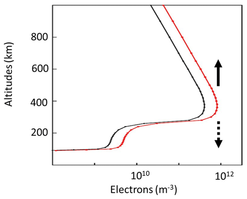
Figure 2Vertical profiles from 90 to 1000 km in altitudes of electron number density in two conditions: pre-onset in black and after accumulation in red. The nighttime sunspot maximum condition given in Prince Jr. and Bostick Jr. (1964) was used to plot the pre-onset condition. Vertical arrows directing upward and downward denote traveling ion acoustic waves propagating along the field lines from the density peak of the F layer.

Download

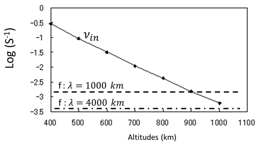
Figure 3Ion-neutral collision frequency (ν_in) in altitudes from 400 to 1000 km calculated using the nighttime sunspot maximum condition in Prince Jr. and Bostick Jr. (1964). Wave frequencies of ion acoustic wave are overlaid for two wavelengths: 1000 and 4000 km along field lines (see text).

Download

Altitude profiles of steady-state ion flows were evaluated substituting 1000 K for ion temperatures and the same e-folding distance in Eq. (4). The ions are oxygen and parallel electric fields are given by the Eq. (4). A snapshot of the velocity profile in altitudes from 400 to 800 km is shown in Fig. 4 for the two cases of electron temperatures: 5000 K for black dots and 1000 K for red dots. For the low-temperature case (1000 K), no ion upflow occurred because the parallel electric fields could not overcome gravity. We suggest that electron temperatures over 2700 K would be needed to excite ion upflow. When electron temperature was set to 5000 K, the ion velocity of 15 m s⁻¹ at 400 km in altitudes increased rapidly to 1369 m s⁻¹ at 800 km. The altitude profile of the flow velocity in Fig. 4 matched type-2 ion outflow observed by the EISCAT radar (Wahlund et al., 1992). We conclude that the ion upflow in topside ionosphere was caused primarily by the parallel electric fields excited by the upward-traveling ion acoustic wave. Below 600 km in altitudes, upflow velocity was 1 to 2 orders of magnitude smaller than the equatorward drift in the flow channel. Upflow velocity became comparable to the horizontal drift over 800 km in altitudes and exceeded the phase velocity of ion acoustic wave. Ion outflow velocity exceeding the phase velocity of ion acoustic wave along the field lines may excite a shock at the topside ionosphere. A part of them developed to ion acoustic double layers (Sato and Okuda, 1980; Hasegawa and Sato, 1982; Hudson et al., 1983; Ergun et al., 2002) which were observed at the altitudes of 6000–8000 km (Mozer et al., 1977; Temerin et al., 1982). Those ion acoustic double layers would have produced parallel potential structures referred to as inverted-V-type electric fields.

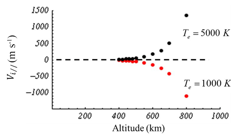
Figure 4Steady-state parallel velocity in altitudes for ions (oxygen) produced by parallel electric fields: 0.4 µV m⁻¹ (T_e=1000 K) in red dots and 2.0 µV m⁻¹ (T_e=5000 K) in black dots. Vertical flows in altitudes from 400 to 800 km are shown. Flow velocity is positive upward and negative downward.

Download

Accumulation of electrons and ions occurred at the equatorward end of the flow channel. We can estimate a rate of accumulation by the following relation:

Here n is plasma density, and U denotes drift velocity in the flow channel in x. Substituting ΔU=10³m s⁻¹ and Δx=10⁴ m, we have $\frac{\mathrm{\Delta }n}{\mathrm{\Delta }t}={\mathrm{10}}^{\mathrm{10}}$ m⁻³ s⁻¹ for the background densityn₀=10¹¹ m⁻³. This gives a density pileup of the order of $\frac{\mathrm{\Delta }n}{n_{\mathrm{0}}}=\mathrm{100}$ % in 10 s. If the equatorward drift in the flow channel is an order of 10³ m s⁻¹ (E=100 mV m⁻¹ in the auroral ionosphere) and electron production by the precipitation does not exceed the accumulation rate, which was 100 % of the background density in 10 s, both outflows and precipitation may not bring significant changes to the flux carried by E×B drift in the flow channel. We then approximate one-dimensional (along the drift path in x) conservation equation in the flow channel.

A question arises regarding maximum accumulation of plasmas at the equatorward end of the flow channel. One possible mechanism to suppress accumulation may be associated with the ionospheric screening that decreased the amplitudes of penetrated (total) westward electric fields by the increasing ionospheric conductivities. In a two-dimensional ionosphere with uniform height-integrated conductivity, total electric fields E given by a sum of the incident (E_i) and reflected westward electric fields may be written as $E=\left(\mathrm{2}{\mathrm{\Sigma }}_{\mathrm{A}}\left({\mathrm{\Sigma }}_{\mathrm{A}}+{\mathrm{\Sigma }}_{\mathrm{P}}\right)\right)E_{\mathrm{i}}$, where Σ_A and Σ_P are the Alfven conductance defined by 1∕μ₀V_A and height-integrated Pedersen conductance in the ionosphere, respectively (Kan et al., 1982). Symbols μ₀ and V_A denote magnetic permeability in vacuum and Alfven velocity, respectively. The amplitude ratio of total electric fields to incident electric fields is a function of the conductance ratio of Pedersen and Alfven; $E/E_{\mathrm{i}}=\mathrm{2}$ for a low conductivity of the ionosphere satisfying ${\mathrm{\Sigma }}_{\mathrm{P}}/{\mathrm{\Sigma }}_{\mathrm{A}}\ll \mathrm{1}$, and $E/E_{\mathrm{i}}=\mathrm{0}$ for a high conductivity of the ionosphere satisfying ${\mathrm{\Sigma }}_{\mathrm{P}}/{\mathrm{\Sigma }}_{\mathrm{A}}\gg \mathrm{1}$. Noting that Σ_P is proportional to the plasma density in the ionosphere, the total electric fields monotonically decreased with increasing plasma densities caused by accumulation itself and by the precipitations associated with the auroral activity. Another explanation may be suggested in the polarization electric fields (eastward) produced by the accumulation itself. These electric fields grew quickly with density accumulation and decreased the incident electric fields (westward) by the superposition. In addition to the above scenarios, we surmise that excess accumulation of the ionospheric plasmas may be suppressed through the term (U⋅∇)U in the equation of motion. From the ionospheric screening process discussed above, we tentatively assume that flow velocity U is a function of the density n. Then the conservation Eq. (7) may be written as

Here, Q(n) is a mass flux defined by Q(n)=nU(n). This relation can be reduced to the nonlinear wave equation,

Here c(n) is a wave propagation velocity defined by $c\left(n\right)=U\left(n\right)+n{U}^{\prime }\left(n\right)$, U(n) is a drift velocity in the flow channel, and U^′(n) denotes braking/acceleration of the drift velocity by increasing and decreasing density. The Eq. (9) is often referred to as propagation of kinematic waves to describe traffic flow (Lighthill and Whitham, 1955). In the following, we use dimensionless units normalized by U_m and n_m. Here, U_m and n_m denote maximum drift velocity at n=0 and maximum density for complete stops of the drift, respectively. Assuming a constant braking in the flow channel, we define U by a linear function of density n as $U\left(n\right)=\mathrm{1}-n$. Noting that $Q^{\prime }\left(n\right)=c\left(n\right)$, this relation is reduced to the equation $Q\left(n\right)=n(\mathrm{1}-n)$, which is identical to the case for the traffic flow (Whitham, 1999). Both the U and Q are plotted in Fig. 5a as a function of n. A nonlinear evolution of the density waves is presented in Fig. 5b by the characteristic curves. In the case of vehicles in traffic, the initial flows started from n=0 and stopped at n=1.0 by the tailback of cars. For the case of the ionosphere, the ionospheric density started from a finite density, n=0.3 in Fig. 5b, and increased to n=1.0 to terminate the flow by the full screening. The nonlinear evolution of the density profile in time is shown in Fig. 5b in colors from black (T=T₁), red (T=T₂), green (T=T₃), blue (T=T₄), and to purple (T=T₅). After T=T₅, the waves propagate upstream (poleward) as a shock. The shock velocity, V, is given as (Whitham, 1999)

Here, subscript 1 is for the values ahead of shock and subscript 2 is for the values behind. Noting that Q(n₂)=0 and substituting $Q\left(n_{\mathrm{1}}\right)=n_{\mathrm{1}}(n_{\mathrm{2}}-n_{\mathrm{1}})$, the Eq. (10) can be reduced to $V=-n_{\mathrm{1}}$ in dimensionless unit. The propagation velocity of the shock is related to the densities ahead. For the case of n=0.3 in Fig. 5b, shock velocity can be estimated to be −0.3U_m. Here, U_m denotes maximum drift velocity in the ionosphere where ionospheric screening effects vanished by the condition ${\mathrm{\Sigma }}_{\mathrm{P}}/{\mathrm{\Sigma }}_{\mathrm{A}}\ll \mathrm{1}$. The shock velocity may be of the order of kilometers per second, which is comparable but opposite to the equatorward drift in the flow channel.

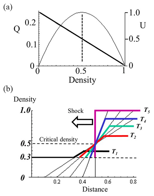
Figure 5(a) Normalized flux (Q)–density (n) curve (thin curve) and velocity (U)–density (n) line (thick line) in flow channel. Vertical scale of the U–n line is shown to the right; the scale of the Q–n curve is to the left. Dotted line at n=0.5 indicates the critical density where c(n) vanishes; waves are stationary relative to the ground. Waves propagate forward/backward at a density below/above the critical density. (b) Nonlinear evolution of the density accumulation. Density increased in a step-like manner from T₁ to T₅.

Download

No data sets were used in this article.

The author declares that there is no conflict of interest.

This paper was edited by Matina Gkioulidou and reviewed by two anonymous referees.