2.1 Principles of single-spacecraft FAC estimation

FAC density estimators can be based on single-spacecraft or multi-spacecraft data (Ritter et al., 2013; Vogt et al., 2013). Here we adopt the single-spacecraft approach to construct a FAC density scalogram, i.e., a multiscale representation of FAC density. Single-spacecraft FAC estimators are based on Ampére's law, $\mathit{j}={\mathit{\mu }}_{\mathrm{0}}^{-\mathrm{1}}\mathrm{\nabla }\times \mathit{B}$, with the field-aligned component given by

For a sufficiently elongated FAC sheet, in the sheet reference system, Eq. (1) reduces to

The typical method used to describe the orientation of the FACs is the MVA (Sonnerup and Scheible, 1998) applied to the magnetic field measurements. MVA is based on the assumption of planarity and stationarity. MVA analysis for FACs can be performed on all components of B (3-D MVA) or, in a simplified case, on the perpendicular perturbation, B_⟂ (2-D MVA). The full 3-D MVA can be applied in any reference frame, e.g., GEO, MFA, and yields λ_min, λ_int, and λ_max associated with the directions along B (e_min), perpendicular (e_int), and tangential (e_max) to the arc, respectively. The 2-D MVA provides only λ_ξ≡λ_int and λ_η≡λ_max associated with the normal (e_ξ) and tangential (e_η) directions to the arc, and is rather limited to MFA frames. The GEO frame requires the 3-D MVA since we do not have a strict alignment of the z axis with B, and part of the variance of ΔB is contained in the parallel component. We note that various other combinations are also possible by imposing constraints on e_min, e.g., aligned with B. In the following we use the subscripts min, int, and max when referring to the 3-D MVA, and ξ and η for the 2-D MVA.

The analysis performed in this paper is done in the MFA coordinates and takes into account only the variance in B_⟂. By using this simplified approach we get a lower variance in the data (not including B_∥) and thus expect better results with respect to the 3-D case. The 2-D approach is particularly useful for the case of small-scale FACs in order to avoid ambiguous cases where e_min is associated with a perpendicular direction rather than with the B_∥ direction. Moreover, we note that at the low-altitude Swarm orbit B_z (or B_ζ) can be affected by large-scale remote current systems in the ionosphere, e.g., the electrojet current. A statistical study emphasizing the global characteristics of the Hall current derived from Swarm observations was performed by Huang et al. (2017).

2.2 FAC density from single- and multi-spacecraft data

In the idealized case of an infinite planar current sheet oriented along the east–west direction (east–west aligned auroral arcs), the FAC density is approximated by discretizing Eq. (1) and by using the spacecraft velocity, v^sc, to compute the spatial gradient along the normal to the FAC structure:

For the quasi-static FAC approximation and in the case of spacecraft crossing along the normal to the arc, Eq. (3) gives correct results. In reality, due to the orbital configuration and FAC dynamics, the crossings are not normal to the arc and the FACs show deviations from the quasi-static approximation. Equation (3) was used to obtain estimates of the FAC density for many single-spacecraft missions like Freja (e.g., Luhr et al., 1996) and FAST (Elphic et al., 1998), or more recently for single-spacecraft FAC estimates from Swarm (Ritter and Lühr, 2006).

For an east–west aligned FAC sheet, the observed sign of the slope in the B_y time series (with the y axis pointing towards east) depends not only on the FAC direction, but also on the direction of the spacecraft velocity V and on the hemisphere. The sign of B_y time series slope equals FAC direction with respect to B₀ (ambient field) for poleward motion, whereas this relation is reversed for equatorward motion. The general algebraic relationship for a sheet with normal unit vector $\widehat{\mathit{n}}$ is

For an ideal (infinitely extended) sheet of FACs, we obtain

since $\dot{\mathit{B}}\times {\widehat{\mathit{B}}}_{\mathrm{0}}$ is aligned with $\widehat{\mathit{n}}$. Hence the FAC is positive/negative if the two vectors $\dot{\mathit{B}}\times {\widehat{\mathit{B}}}_{\mathrm{0}}$ and V form an angle smaller/larger than 180^∘. Note that in the Northern Hemisphere, positive FACs are downward currents and negative FACs are upward currents. In the Southern Hemisphere, negative FACs are downward currents and positive FACs are upward currents. In Sect. 4 we show events with both poleward and equatorward crossing by Swarm spacecraft.

When multi-spacecraft information is available, one can relax part of the assumptions involved in the single-spacecraft methods to compute the FAC density. For the case of the Swarm mission, the multi-point configuration is constructed by using the low orbit SwA and SwC spacecraft. By shifting the along-track positions one can build virtual quads which make an appropriate configuration for the computation of the FAC density. Based on their computation principle, we distinguish two classes of dual-spacecraft methods. Finite differencing (FD) methods (Ritter et al., 2013; Ritter and Lühr, 2006) evaluate a discrete version of the boundary integral $j_{\parallel }=({\mathit{\mu }}_{\mathrm{0}}A{)}^{-\mathrm{1}}\oint \mathit{B}\cdot \mathrm{d}\mathit{s}$. Linear least squares (LS) estimators (Vogt et al., 2009, 2013) are constructed by projecting the dual-satellite measurements onto a local linear magnetic field model.

While both FD and LS methods have obvious advantages over the single-satellite methods, they are limited with respect to the scale resolution. The along-track separation can be varied in order to obtain squared quads configurations, whereas the cross-track is limited by the orbit separation. Thus, the cross-track separation defines the lower limit of the FAC scales in the cross-track direction, whereas the limit in the along-track direction is determined by the along-track separation, provided that the FAC structure is quasi-stationary. The typical cross-track separation between SwA and SwC above the auroral oval is decreasing towards poles from ∼80 to ∼50 km around latitudes of ∼60 to ∼70^∘, respectively. The along-track separation of about 10 s corresponds to some 70 km.

2.3 Multiscale FAC density scalogram

In order to characterize the small-scale FACs, one has to rely on single-spacecraft methods. Bunescu et al. (2015) introduced the multiscale FAC analyzer (MSMVA) to study the FAC signatures. The MSMVA technique extends the MVA analysis by providing continuous and multiscale information on the planarity and orientation of the observed FACs. The continuous character over the time domain is achieved by computing the MVA parameters (eigenvalues and eigenvectors) over a sliding window (width w). The multiscale character is achieved by repeating the procedure for an array of window widths, w_k, within a given range (resolution dw). The eigenvalues (λ_η, λ_ξ), eigenvectors (e_η, e_ξ), eigenvalues ratio, $R={\mathit{\lambda }}_{\mathit{\eta }}/{\mathit{\lambda }}_{\mathit{\xi }}$, and the orientation, θ≡  $({\mathit{e}}_{\mathit{\xi }},\widehat{\mathit{x}})$, are thus 2-D quantities dependent on time and scale. Bunescu et al. (2015) showed that the derivative of λ_η with respect to the length of the analysis window, ∂_wλ_η, provides the location (center) and scale (thickness) of the planar FAC structures. We note that the amplitude of ∂_wλ_η depends on the scanning parameter w which represents the along track scale. In order to obtain the amplitude corrected derivative we use the orientation information, ${\partial }_{\mathit{\xi }}{\mathit{\lambda }}_{\mathit{\eta }}={\partial }_w{\mathit{\lambda }}_{\mathit{\eta }}/\cos \left(\mathit{\theta }\right)$. Here after in this work we only use the amplitude corrected derivative ∂_ξλ_η.

The method was checked on simple synthetic FACs (infinite and finite structures) of both uniform and nonuniform FAC density and showed good performance in identifying FAC scales. The method was applied to Cluster data showing both large-scale quiet arcs and locally planar and dynamic FAC structures (Bunescu et al., 2015), as well as for the analysis of conjugate Cluster/FAST observations (Bunescu et al., 2017).

The multiscale information provided by MSMVA can be used to compute other quantities, like the FAC density. MSMVA provides the scale-dependent orientation that can be used to compute the FAC density in the FAC's own reference system. Combined with the MSMVA results this provides a consistent tool to analyze the FAC signatures. One can compute the FAC density at each scale by discretizing Eq. (2):

where B_η is computed as the projection of B along the tangential direction, $B_{\mathit{\eta }}=\mathit{B}\cdot {\mathit{e}}_{\mathit{\eta }}$, whereas Δξ is the thickness across the structure in the normal direction. Assuming a certain velocity of the spacecraft, v_sc, Δξ can be computed by using the projection of v_sc on e_ξ and the spacecraft crossing times, $\mathrm{\Delta }\mathit{\xi }={\mathit{v}}_{\mathrm{sc}}\cdot {\mathit{e}}_{\mathit{\xi }}\mathrm{\Delta }t$. We note that Eq. (6) provides the amplitude corrected FAC density because at each scale j_∥ is computed by taking into account the perpendicular scale variation, Δξ.

The amplitude of B_η at each scale w=Δt is estimated by fitting B_η using a simple linear regression analysis. Thus, $\mathrm{\Delta }{B}_{\mathit{\eta }}=B_{\mathit{\eta }}\left(t_b\right)-B_{\mathit{\eta }}\left(t_a\right)$, where t_a and t_b are the limits of the analyzing window, w, at the respective position (center t_cen of [t_a, t_b] interval). When the analyzing scale is centered on a certain FAC structure and has the width equal to the FAC thickness, ΔB_η approximates well the entire perturbation across the structure. When the analysis window is centered between two balanced FACs of similar amplitude, j₀, and thickness, w₀, the two FACs cancel each other and provide no contribution to the current at that position and scale, ΔB_η=0. In the case of unbalanced FAC structures, the FAC density depends on their respective amplitudes and thicknesses.

The ensemble of the resulting estimates $j_{\parallel }=j_{\parallel }(t_{\mathrm{cen}},w)=j_{\parallel }(t_{\mathrm{cen}},\mathrm{\Delta }t)$ yields a multiscale representation of FAC density in (t_cen,w) space. We refer to this graphical representation as the FAC density scalogram, in analogy to the terminology used for wavelet transforms (Torrence and Compo, 1998).

The multiscale information can be separated into invariant information, which depends only on quantities in the local (ξ, η) frame, and non-invariant information, which depends also on variables in the (x, y) frame. All multiscale information depends on w, which is the scale length along the spacecraft track ((x, y) frame) and thus a non-invariant variable. In order to obtain the dependencies on the perpendicular scale (FAC thickness), one has to correct the scale array w_k by projection along the $\widehat{\mathit{\xi }}$ direction, w_kcos (θ_k). Regarding the amplitude of the MSMVA quantities, we notice that invariant information is given by R_λ and θ, but non-invariant information by uncorrected j_∥ and ∂_wλ_η. Corrections to the scale are applied for the individual profiles (dependence at a certain time or position; see Sects. 3 and 4) and not to the scalograms of MSMVA quantities. As long as both synthetic and observed FACs are essentially east–west aligned (Bunescu et al., 2015), the method cannot be properly tested and validated for inclined structures. In Sect. 3 we perform tests on inclined synthetic FACs, whereas in Sect. 4 we also apply the method to inclined FAC observations by Swarm.

2.4 Scale sampling schemes

We use two different FAC scanning procedures (scaling schemes) for the discretization of the FAC scale domain. The scheme implemented by Bunescu et al. (2015) implies a linear sampling of both scale and time domain, i.e., linearly varying width for scale space and sliding for the time space. At a given time the discretization of the scale domain is similar to the nested MVA analysis (Sonnerup and Scheible, 1998) used to study the stationarity of the MVA parameters. The minimum scale, w_min, is given by three points (one point on each side of the central point). Iteratively, the scale increases by adding an equal number of points (depending on dw resolution) to the sides of the previous scale, yielding thus an array of odd numbers w_k=3, 5, 7, … for the highest-resolution scanning. For the Swarm high-resolution magnetic field data (Sect. 4) we look in the range between w_min=0.1 s and w_max=5 min, which for an ionospheric mapping factor of 1.1 corresponds roughly to an ionospheric scale of about ∼760 m and ∼2000 km, respectively. This scheme has the advantage that one can scan all the FAC scales present in the data and provide the high resolution needed in the FAC scale/position identification (Bunescu et al., 2015). As discussed in Sects. 3 and 4, this high-resolution linear scanning introduces a large degree of correlation in the results. Indeed, for an infinite planar sheet of width w₀, this is sampled many times for all scales w_k≤w₀. When searching for FAC scale/location this proved to be fine, since ∂_wλ_η maximized at w₀ for essentially east–west aligned FACs.

The second FAC scanning scheme uses successive intervals that do not overlap at a certain scale; the length of the intervals is varied logarithmically to provide information at different scales. This scheme is similar to the one used in Haar wavelet decomposition. All scales (interval widths) spanning w_k=2^k data points, where k=2, N (N the highest power of 2 that fits into the data interval) are considered. When dealing with large scales one can use zero padding of the data interval. Practically, in an ideal auroral oval configuration with balanced R1/R2 FACs, the largest scale samples the entire oval, and in the second-largest scale the interval is split into two and addresses separately the R1/R2 regions. The segmentation of the data interval repeats down to the smallest-scale w_min. For the case of Swarm events (Sect. 4) we take w_min=0.04 s (two points) and w_max=21.8 min corresponding to a total number of 16 decomposition levels. One sensitive point of this scheme is the centering of the data interval because in reality we do not have an ideal oval; e.g., one can have a tangential crossing through the oval. One can manually center the analysis interval on the border between the R1 and R2 regions. The main advantage of this logarithmic scheme is that it is much faster than the linear scheme and provides a more intuitive understanding of the multiscale FAC density. In each computation cell of width Δξ^(k) we have the current density $j_{\parallel }^{\left(k\right)}={\mathit{\mu }}_{\mathrm{0}}^{-\mathrm{1}}\mathrm{\Delta }{B}_{\mathit{\eta }}^{\left(k\right)}/\mathrm{\Delta }{\mathit{\xi }}^{\left(k\right)}$ and the integrated current $J_{\parallel }^{\left(k\right)}={\mathit{\mu }}_{\mathrm{0}}^{-\mathrm{1}}\mathrm{\Delta }{B}_{\mathit{\eta }}^{\left(k\right)}$. The FAC density $j_{\parallel }^{\left(k\right)}$ reflects the slope of B_η, whereas $J_{\parallel }^{\left(k\right)}$ reflects the jump of B_η over the respective scale, w_k. Both $j_{\parallel }^{\left(k\right)}$ and $J_{\parallel }^{\left(k\right)}$ offer complementary useful information. In the following we concentrate on $j_{\parallel }^{\left(k\right)}$, similar to the linear sampling scheme.

As it is constructed, the multiscale FAC density provides estimates of the average FAC across scales, as well as an indication of the dominant scales, given by peaks in ∂_ξλ_η. Both scale sampling schemes rely on non-orthogonal basis functions because the aim is to precisely infer the scale and location of the FAC as well as the respective current density. As a consequence, one cannot simply integrate over scales to obtain a global FAC density estimate that can be compared with the single- and dual-spacecraft FAC estimates – which provide convoluted information about the FAC scales larger than the discretization interval (single-spacecraft) or the virtual quad scale (dual-spacecraft). As compared to the orthogonal decompositions, e.g., orthogonal wavelet decomposition, where the signal is recovered easily by integration over scales, in our case such an integration would require a proper weighting scheme of the multiscale information. This development is considered for a future study.

3.1 FAC structure of balanced current

In the following we consider the current system consisting of the downward/upward (labeled FD/FU) current regions. The value of the thickness parameter, σ_⟂, for both FAC structures is 50 km. Typical values of ΔB for the auroral region are in the range of a few 100 nT. Each 100 nT in the measured ΔB corresponds to an integrated sheet current J₀∼0.1 A m⁻¹. For this synthetic case we consider $J_{\mathrm{0}}=\pm \mathrm{0.63}$ A m⁻¹ for the downward/upward current. The current elements are located at $x_{\mathrm{0}}^{\left(\mathrm{1}\right)}=\mathrm{600}$ and $x_{\mathrm{0}}^{\left(\mathrm{2}\right)}=\mathrm{800}$ km. We introduce a variation of the orientation from ${\mathit{\theta }}^{\left(\mathrm{1}\right)}=\mathrm{0}{}^{\circ }$ at FD to ${\mathit{\theta }}^{\left(\mathrm{2}\right)}=\mathrm{40}{}^{\circ }$ at FU. According to observations (Gillies et al., 2014) the value of ${\mathit{\theta }}^{\left(\mathrm{2}\right)}=\mathrm{40}{}^{\circ }$ is a rather extreme case for a stable auroral arc.

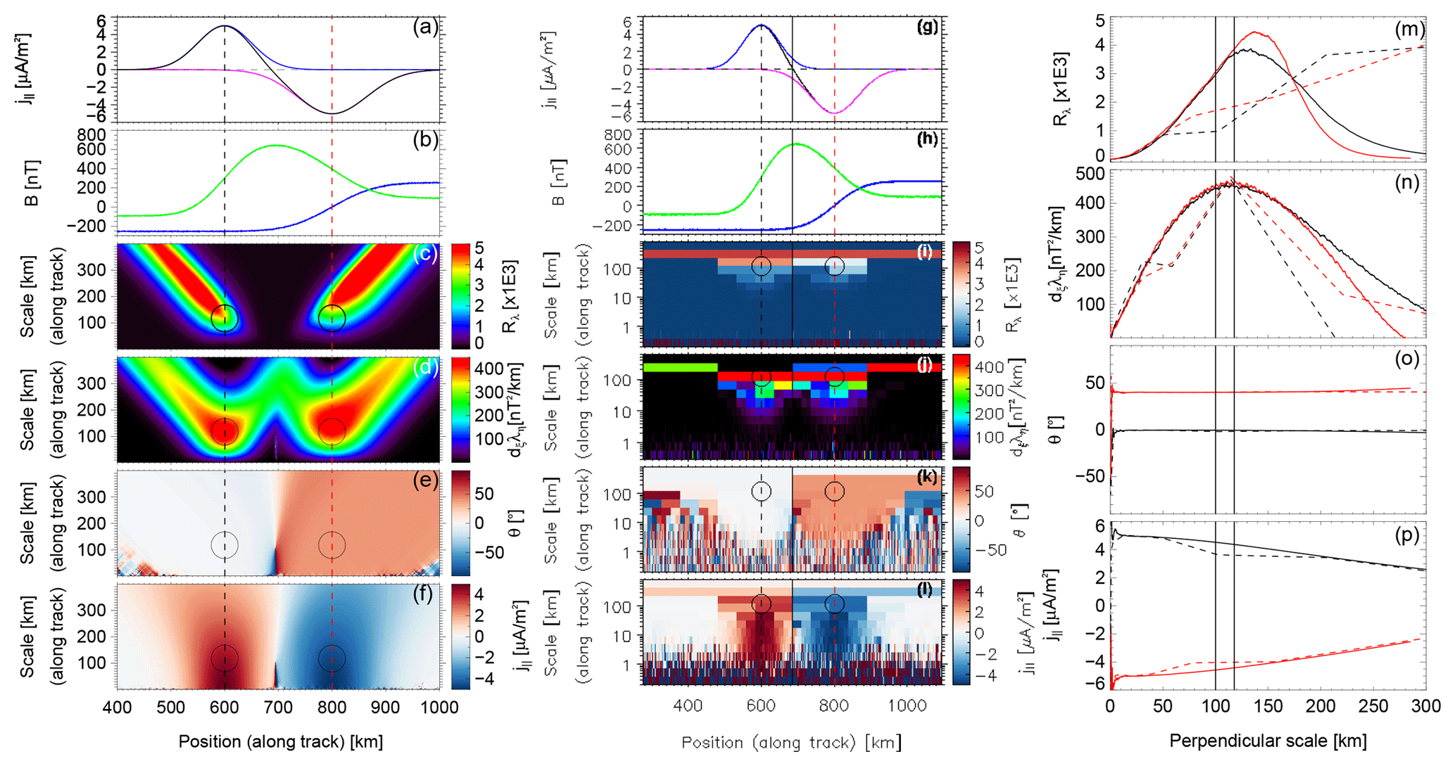
Figure 1MSMVA analysis for the linear and logarithmic scheme. (a) Input FAC density for FD (magenta), FU (blue) and the summed contribution from both FACs (black); (b) magnetic field perturbation in the (x, y) frame with B_x (blue) and B_y (green); (c) planarity, R_λ; (d) FAC scale/location, ∂_ξλ_η; (e) orientation, θ; (f) multiscale FAC density; panels (g)–(l) show the same quantities for the logarithmic sampling scheme. Panels (m)–(p) show the profile of R_λ, ∂_ξλ_η , θ, and j_∥ at the center of FD/FU structures indicated by the vertical black/red dashed lines in panels (a)–(f) and (g)–(l). The vertical black lines indicate w_1σ and fwhm scales discussed in the text. Solid/dashed lines indicate the profiles for the linear/logarithmic scanning.

Download

Figure 1 shows the results of both linear- and logarithmic-scale sampling for this simple FAC structure. Panel (a) shows the input current density, j_∥, of FD (magenta), FU (blue), and the total current (black). Panel (b) shows the B_x (blue) and B_y (green) components of the obtained magnetic field (Eq. 11). This magnetic field contains a superposed normal distributed noise signal with zero mean and sigma of 3 nT. The maximum FAC density at the center of the two structures is ∼5 µA m⁻². The results of linear MSMVA scanning of the FAC system are shown in panels (c), (d), (e), and (f) by the planarity R_λ, the derivative ∂_ξλ_η, the orientation θ, and the linear multiscale FAC density, respectively. The width array used in the linear MSMVA is between 1 and ∼400 km with a step of ∼0.6 km. We note the smooth variation of all quantities specific to this sampling scheme. On each spectrum we indicate the position and scale or the input FACs by the black circles (diameter equal to σ_⟂). ∂_ξλ_η correctly identifies the scale of FD around fwhm =117 km. For FU we get a larger estimate because of the dependence of ∂_ξλ_η on the non-invariant w variable (length along the track). The sections at the FAC centers shown below are represented as a function of the corrected scale, obtained by projection of the scale array on $\widehat{\mathit{\xi }}$ using the orientation (Sect. 2.3). θ scalogram (panel e) correctly identifies the orientation, ${\mathit{\theta }}^{\left(\mathrm{1}\right)}=\mathrm{0}{}^{\circ }$ and ${\mathit{\theta }}^{\left(\mathrm{2}\right)}=\mathrm{40}{}^{\circ }$. We note that R_λ shows a signature with a rather flat maximum extending to large scales, with the local maxima for FD/FU regions not coincident with ∂_ξλ_η maxima. This behavior is influenced by the smoothness of ΔB for each FAC and by the constant ΔB located before/after FD/FU FACs. The multiscale FAC density shows higher values at smaller scales, roughly up to the actual scale of the structure, and decreasing values above this scale – indicated by ∂_ξλ_η. This can be understood by considering the simple example of a uniform current sheet: the current density remains constant for all the scales smaller than the sheet width and decreases asymptotically to zero for larger scales. The panel on current density provides scale information just qualitatively. The quantitative aspect is addressed in correlation with the corrected ∂_ξλ_η information shown in sections at specific times (see right panels of Fig. 1).

Panels (g)–(l) show the results of logarithmic FAC scale scanning. For this case the analysis is centered in the middle of the FAC structure, indicated by the vertical black line. The sampled scale array covers 13 logarithmic levels from w_min=0.2 to w_max=820 km. The logarithmic scheme shows a more discrete character due to the non-overlapping sampling intervals at each scale. Qualitatively, we observe a good agreement with the linear scheme for the orientation (panel k) and FAC density (panel l). The multiscale FAC density (panel l) shows at the largest scale a close to zero current because the two structures have similar amplitudes and compensate each other. At around 100 km we observe the separation of the two branches of the current centered at 600 and 800 km. The distinction between the two regions is very clear down to smaller scales of a few kilometers. Higher FAC intensity is observed around the centers of the FACs for scales smaller than about ∼50 km.

Quantitative estimates are obtained trough vertical cuts into the MSMVA scalograms shown in panels (m)–(p) of Fig. 1. The black/red line shows the profiles in the center of FD/FU structures, whereas the solid/dashed lines indicate the results for the linear/logarithmic sampling scheme. The vertical dashed lines show the scales w_1σ=100 km and fwhm =117 km. As discussed in Sect. (2.3), for all multiscale parameters we correct the scale variable (multiplication of the scale array by cos(θ)) to get the dependence on the perpendicular scale. For both FACs ∂_ξλ_η (n) shows that the scale is more consistent with fwhm estimate. We notice that for this simple FAC system both the linear and logarithmic sampling scheme provide consistent results, the scale is precisely identified in both cases. The orientation of the two FACs (o) at fwhm scale is consistent with the input parameters, 0^∘ and 40^∘ for FD and FU, respectively. We note that the scale corrected ∂_ξλ_η does not depend on the FAC's orientation. The similarity of ∂_ξλ_η amplitudes for FD and FU indicates a good amplitude correction for FU structure. R_λ profile (m) does not have a maximum at the same scale as ∂_ξλ_η. This shift is dependent on the noise level since R_λ contains also dependence on λ_ξ. The local FAC density (p) at FD and FU locations provides also quantitative indication about the FAC scale. Around the FAC scale we observe a slight change of the slope of j_∥ for the linear scheme and also a decrease for the logarithmic scheme. At a given FAC center j_∥ shows a rather constant plateau and starts to decrease when the scanning reaches its characteristic scale. This behavior is more evident for uniform FAC density structures (see Sect. 4.2). The FAC density for FD and FU FACs shows values of about ±4.5 and $\sim \pm \mathrm{3.5}$ µA m⁻² for the linear and logarithmic sampling, respectively, i.e., 10 % and 30 % smaller than the input FAC density (5 µA m⁻²).

3.2 Superposition of Gaussian FAC structures

We start again with a large-scale current system similar to the previous synthetic case. Two FAC elements FD and FU with ${\mathit{\sigma }}_{⟂}^l=\mathrm{50}$ km and $J_{\mathrm{0}}^l=\pm \mathrm{0.63}$ A m⁻¹ are placed at x₀=700 and x₀=900 km. The orientation of FD and FU structures is ${\mathit{\theta }}_l^{\left(\mathrm{1}\right)}=\mathrm{0}$ and ${\mathit{\theta }}_l^{\left(\mathrm{2}\right)}=\mathrm{40}{}^{\circ }$. A number of three small-scale FACs are superposed on each large-scale FAC structure. We consider equal scales of the embedded FACs given by ${\mathit{\sigma }}_{⟂}^s=\mathrm{5}$ km. The small-scale FACs embedded in FD have $J_{\mathrm{0}}^{\left(k\right)}$ parameters defined as $J_{\mathrm{0}}^l/\mathrm{6}$, $J_{\mathrm{0}}^l/\mathrm{3}$, and $J_{\mathrm{0}}^l/\mathrm{6}$, alternatively positive and negative. Similarly the small-scale FACs superposed onto FU also have a central more intense FAC of amplitude $J_{\mathrm{0}}^l/\mathrm{4}$ and two side FACs of intensities $J_{\mathrm{0}}^l/\mathrm{8}$. For simplicity, we consider all small-scale FACs to have ${\mathit{\theta }}_s^{\left(k\right)}=\mathrm{0}$^∘. The small-scale FACs introduce alternatively positive and negative amplitude changes in the current density of the large-scale FAC system.

Figure 2Same panels as in Fig. 1.

Download

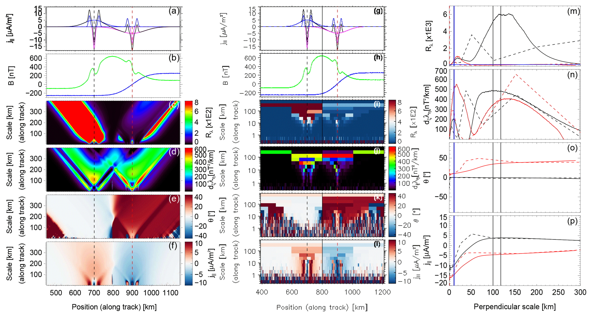
Figure 2 shows the overall contribution of the two scales to a rather complex FAC density profile shown by the black line in panel (a) and the corresponding magnetic field perturbation in panel (b). The FAC elements are indicated in panel (a) with blue/magenta for the positive/negative FAC densities at both scales. The attenuation (compensation)/intensification (addition) of the local FAC density from the two FAC systems is reflected in slower/steeper gradients of ΔB. We note that the superposition of scales (Eq. 11) affects the orientation and the scale information for both large- and small-scale FACs. Thus, in general we do not expect to find the exact input angles and scales. The superposed normal distributed noise signal has σ=2 nT in this case. In this example we perform the linear FAC scanning over the range between 1 and 400 km, but the logarithmic scanning over the scale domain from 0.2 up to 820 km. The total number of levels in the logarithmic scanning is k=13.

Panels (c)–(f) and (i)–(l) show the MSMVA decomposition into the linear and logarithmic schemes, respectively. We notice the same characteristics of the two schemes, namely smooth and coarse results in the linear and logarithmic scannings, respectively. Panel (c) shows a high decrease in the planarity level for FU as compared with the previous case (Sect. 3.1). We note regions of high R_λ at both large- and small-scale FAC systems. The relative combination of angles and amplitudes of B from the two scales leads to three signatures of high R_λ for the small-scale FAC system inside FD, whereas for FU R_λ is high only for the central more intense small-scale FAC. The ∂_ξλ_η scalogram clearly shows the two FAC systems. Besides the signatures around expected scales we also have an intermediate false level of identified FACs caused by the combination of adjacent small-scale FAC elements. In the logarithmic scanning, R_λ (i) and ∂_ξλ_η (j) provide consistent information with the linear scanning. The θ scalograms (e and k) show well the overall structure of the FAC system, with values consistent with ${\mathit{\theta }}_l^{\left(\mathrm{1}\right)}=\mathrm{0}$ and ${\mathit{\theta }}_l^{\left(\mathrm{2}\right)}=\mathrm{40}$^∘ for the large-scale FAC system. At small scales, the variations are related to the vector addition (Eq. 11). While the small-scale FACs inside FD show consistency with the input, θ=0^∘, for the FU region we have good agreement with the input only for the central small-scale FAC, associated with a steeper gradient in B. In the regions of FAC attenuation (weaker gradient) the angles are not consistent with the input orientations, in agreement with the weaker signatures in R_λ and ∂_ξλ_η.

The local FAC density scalogram in both scanning schemes (f and l) provides a consistent view of the input FAC density, with well-delimited FAC elements of both the large- and small-scale FAC systems. In panels (m)–(p) we show vertical cuts through the scalograms at the centers of attenuation/intensification of the FD/FU FAC density by the superposition of the two scales, indicated by vertical dashed lines in panels (a)–(l). The profiles show a more complex situation with respect to the previous synthetic case. The input scales of the two FAC systems are indicated by the vertical black (large scales) and blue (small scales) lines at w_1σ and fwhm. We observe a good correlation of R_λ and ∂_ξλ_η maxima for the small-scale FACs. ∂_ξλ_η shows well-defined peaks for the small-scale FACs consistent with the input scales, but for the large-scale FACs rather broad maxima, also around the expected scales. The orientations are roughly consistent with the input setup, ${\mathit{\theta }}_l^{\left(\mathrm{1}\right)}=\mathrm{0}$^∘ for FD and ${\mathit{\theta }}_l^{\left(\mathrm{2}\right)}=\sim$37–42^∘ for FU. At small scales we also have consistency, ${\mathit{\theta }}_s^{\left(\mathrm{1}\right)}=\mathrm{0}$ and ${\mathit{\theta }}_s^{\left(\mathrm{2}\right)}=\sim \mathrm{5}$^∘ for the small-scale FACs inside FD and FU, respectively. The local FAC density for FD/FU is 4 µA m⁻² ∕ −4.5 µA m⁻², in good agreement with the input of ±5 µA m⁻². For the small-scale FACs centered on FD/FU we have −10 µA m⁻² ∕ −15 µA m⁻², which is roughly consistent with the input FAC density of $\sim -\mathrm{16}$ µA m⁻² ∕ −12 µA m⁻². We get higher/lower deviations for the small-scale FACs centered in FD/FU, in agreement with their weaker/stronger signatures in ∂_ξλ_η.

In the case of superposed FACs the signatures of both large- and small-scale FACs are qualitatively reflected by the MSMVA information. The results also show some limitations of the method. One cannot expect to find a perfect decomposition of the FAC system, because of (a) the use of piece-wise linear functions of a certain length (scale) with a corresponding FAC density profile given by a step function, which is not fully suitable for the smooth Gaussian functions; and (b) the results are actually dependent on the relative parameters (e.g., intensities, orientations, scales, locations) of the superposed FAC elements.

The combined use of R_λ, ∂_ξλ_η, θ, and j_∥ scalograms allows the identification of the geometry, scales, orientations, and estimates of the local FAC densities present at the respective scales. The linear approach shows a high precision in the identification of both FAC scale (d) and local FAC density (f). The logarithmic scheme lacks resolution in the FAC scale identification and subsequently gives a poor estimate of the local current. However, this scheme provides quick results that capture qualitatively similar features. More advanced data processing can include, e.g., filtering ∂_ξλ_η by the planarity R_λ, to remove non-planar FAC structures, and applying a similar mask to current density.

A more systematic study of superposed FAC sheets is required, e.g., by varying the relative parameters of a FAC system consisting of broad and narrow FAC sheets. In this context, we note that a better approach might be to iteratively identify the FACs based on their intensity and to apply MSMVA to the successive residuals obtained by separating the identified FAC signatures (fitting the data at each iteration by model FAC functions, e.g., planar FACs, as indicated by the MSMVA parameters). However, the problem might not be uniquely determined, and before engaging in such a development, we rather apply the present procedure to several real events, three of which are detailed in the next section.

4.1 Instrumentation and basic data processing

The Swarm mission (Friis-Christensen et al., 2008; Olsen et al., 2013) consists of three spacecraft equipped with identical instruments and placed on polar orbits. The primary objective of the Swarm mission is to study the Earth's magnetic field, e.g., mapping, modeling, or separation of the different sources of the measured field. The satellites are equipped with both a vector field magnetometer (VFM) and an absolute scalar magnetometer (ASM) (Hulot et al., 2015) which provide high-accuracy and high-resolution magnetic field measurements. ASM data are used mainly for the calibration of VFM.

In this work we mainly use the VFM measurements to study the FACs. Because we address the multiscale aspect of the FAC signatures and in order to have good statistics also at smaller scales, we use the highest-resolution data provided by VFM, namely the 50 Hz data (0.02 s sampling). The resolution of the data is directly related to the scale of the structures that can be resolved by MSMVA. For a minimum scale of five points in the MSMVA analysis, we obtain an along-track scale mapped to the ionosphere of about 700 m (spacecraft velocity of 7.6 km s⁻¹ and linear mapping factor of ∼1.09).

One major point of the Swarm constellation is its orbital configuration. Two spacecraft, SwA and SwC, are flying side by side at 460 km altitude with a cross-track separation (longitudinal separation) of 1.4^∘ which amounts to about 50–80 km above the auroral oval. The measurements provided by these satellites are combined in the two-satellite methods to estimate the FAC density (Ritter and Lühr, 2006; Ritter et al., 2013). The other spacecraft, SwB, is flying at higher altitude and periodically forms a close three-satellite configuration with the lower pair. When this is the case, it is possible to compute the FAC density by using also a three-spacecraft method (Vogt et al., 2009). In the following, for each event we cross-check the local FAC density provided by MSMVA with the single- and dual-spacecraft estimates.

The single- and dual-spacecraft FAC estimates provided by ESA (part of the Swarm L2 products available at ftp://swarm-diss.eo.esa.int/, last acces: June 2018) are based on the FD approach and available with 1 s resolution. The single-spacecraft FAC density corresponds to a resolution of the mapped ionospheric scale of ∼7 km. The computation of the FD dual-spacecraft FAC estimate is done with a filtered magnetic field perturbation. The filtering is used to remove the FACs with scales smaller than ∼20 s, corresponding to along-track scales smaller than ∼150 km (Lühr et al., 2016). Thus, we expect a good agreement between the single- and dual-spacecraft FAC density estimates for scales larger than 150 km.

The second type of data used in this study is provided by the THEMIS ASI ground network. THEMIS ASI network (Donovan et al., 2006; Mende et al., 2009) was installed to complement spacecraft observations, in particular by the THEMIS mission, related to substorms and, more generally, to auroral phenomena. With a number of 22 stations, the network covers a large region of northern Canada, Alaska, and Greenland. The THEMIS ASI locations were chosen based on an earlier statistical study (Frey et al., 2004) of the auroral substorm onsets inferred from IMAGE spacecraft. Each ASI provides frames of 256×256 pixels at a time resolution of 3 s (exposure time 1 s). All ASI are based on fish-eye lenses that provide wide angle optical observations. Due to the fish-eye lenses the pixels at the center cover a smaller sky surface element as compared to the pixels located towards the edges. Thus, the best resolution is at the center, of about 1 km. The events included in this study make use of optical data from Sanikiluaq (SNKQ), Rankin Inlet (RANK), and Fort Smith (FSMI).

One basic operation is the mapping of the spacecraft orbit into the image plane, done by using the THEMIS TDAS software (http://themis.ssl.berkeley.edu/, last access: June 2018) where the field line tracing is implemented by different versions of the Tsyganenko magnetic field model. In this paper we use the Tsyganenko T04 model (Tsyganenko and Sitnov, 2005) with the solar wind parameters provided by OMNI (http://omniweb.gsfc.nasa.gov, last access: June 2018) and the DST index from WDG at Kyoto (http://wdc.kugi.kyoto-u.ac.jp/, last access: June 2018). The footprints of Swarm are projected onto the optical frames provided by the THEMIS ground stations.

The measured magnetic field is transformed to the MFA reference system. The magnetic field perturbation, ΔB, is obtained by subtracting a model magnetic field from the measured data. The internal magnetic field parameterization is taken from CHAOS-6 (Olsen et al., 2014; Finlay et al., 2016), whereas the lithospheric (e.g., crust and uppermost mantle) and external magnetospheric (e.g., ring current) contributions are taken from the Pomme 10 (Maus et al., 2006, 2010) model. The results obtained for various events in different geomagnetic conditions showed good consistency when using this setup. Ideally, after the subtraction of the magnetic field model we should remain with the perturbation caused by the large-scale R1/R2 currents, the embedded mesoscale and small-scale FACs, as well as the influence of the ionospheric current systems. Another option is to separate the embedded small-scale FACs from the large-scale FACs (R1/R2) by filtering the data. Bunescu et al. (2015) computed a model magnetic field proxy from the measured field using an average over a sliding window (with tapering at the ends). This procedure excludes roughly the scales larger than a certain percent of the sliding window width (depending on the tapering extent). The disadvantage of this approach is that it can introduce additional low-amplitude fluctuations. Thus, in the following we analyze ΔB obtained by subtracting the model magnetic field.

4.2 Stable east–west aligned aurora of constant FAC density

On 17 February 2015 the Swarm spacecraft crossed the auroral oval toward north over the FoV of the SNKQ station. The event is observed around 03:25 UT at ∼1 h after an intermediate substorm intensification/onset following ∼6 h of quasi-steady magnetospheric convection. The AE index is ∼200 nT, and DST $\sim -\mathrm{26}$ nT.

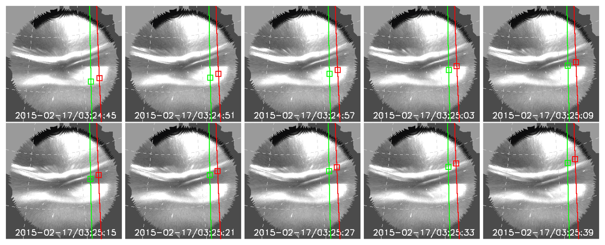
Figure 3Optical frames from SNKQ station mapped in geographic coordinates. The tracks show the ionospheric projection of SwA (green) and SwC (red). At the time of the frame the spacecraft mapped position is shown by the square symbols. The time is overplotted on each frame and covers the interval from 03:24:45 to 03:25:39.

Download

Figure 3 shows the ionospheric footprints of the spacecraft (mapped at 110 km altitude) superposed on the SNKQ optical observations. The optical frames are mapped to geographic coordinates and show rather stable and east–west elongated arc structures. We distinguish two large-scale upward FACs located northward and, respectively, southward of the station. Between these two upward FACs we observe a mesoscale upward FAC with an east–west extent covering the westward FoV of SNKQ. Swarm crosses along the westward edge of the ASI over all three visible arcs. While the thick northward and narrow mesoscale structures are highly planar, the thick southward structure looks curled around the spacecraft tracks. Because Swarm crosses near its center, the magnetic field perturbation for this structure looks similar to that of a planar FAC.

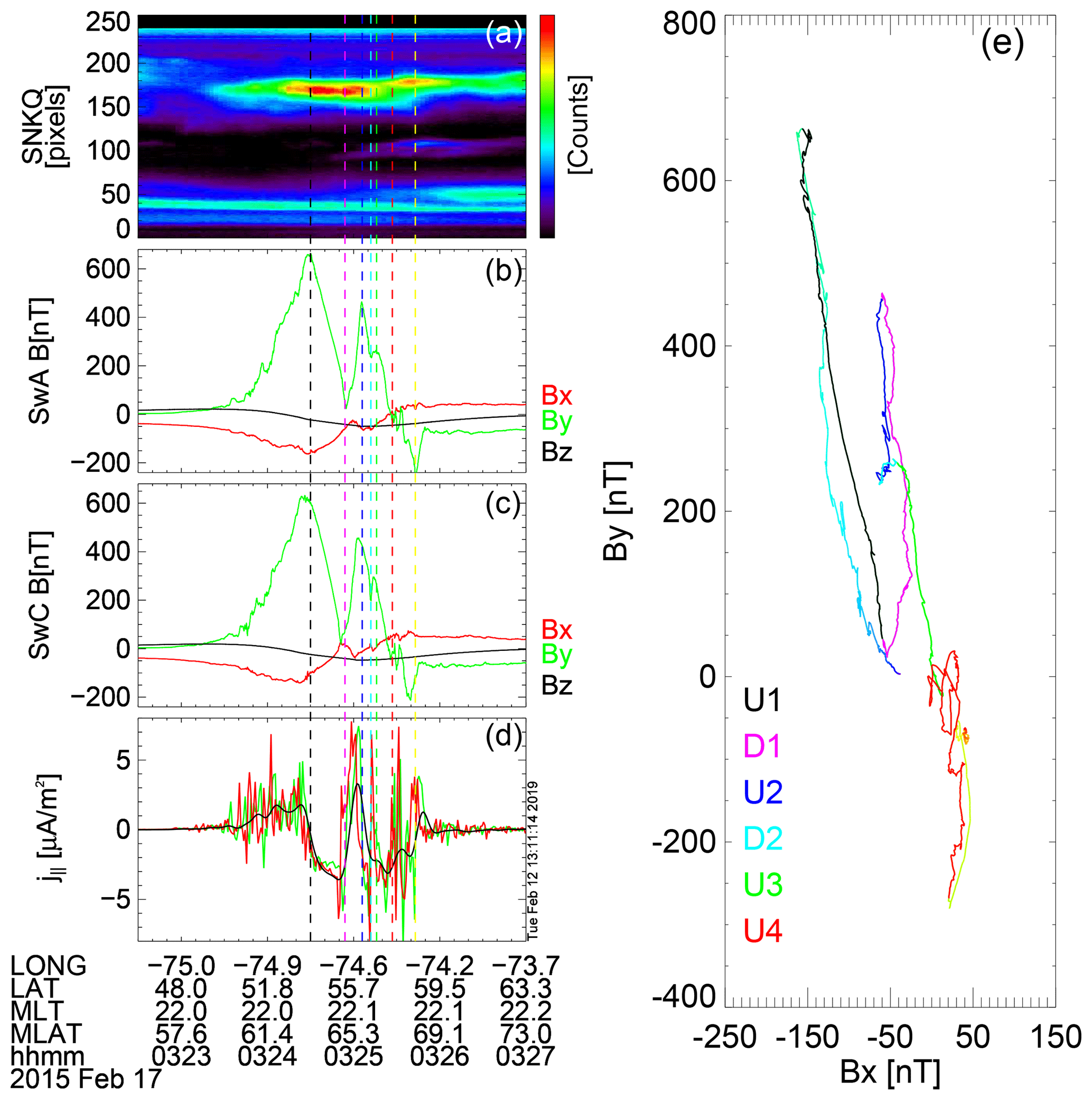
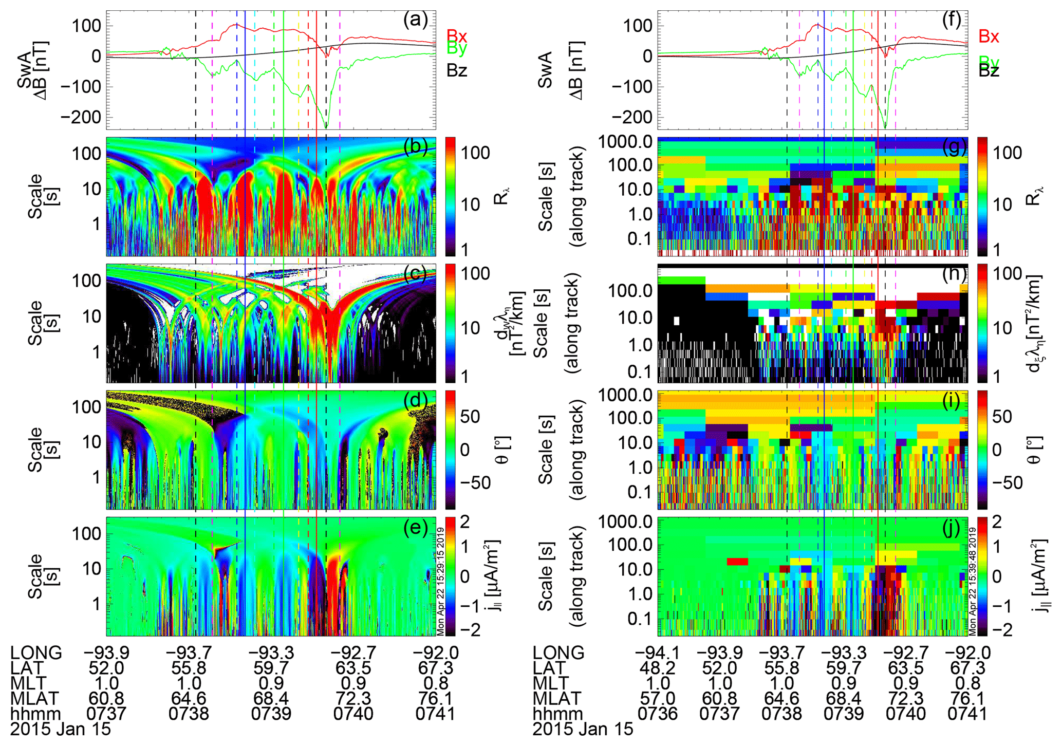
Figure 4(a) Keogram from SNKQ station; (b–c) magnetic field perturbation from SwA and SwC. (d) Single-spacecraft FAC density estimated by the FD method (L2 product) on SwA (green) and SwC (red); the FAC density estimate based on the two-spacecraft FD method (L2 product) is shown by the black line. The vertical dashed lines indicate the beginnings of various FAC elements. (e) Hodogram representation of B_⟂. The hodogram is first represented in a rainbow color scale (blue to red) on which we superpose a layer of identified FAC intervals using discrete colors associated with the labels. For each FAC segment we use the same color as in panels (a–d) to indicate the beginning of the respective FAC element. The U and D labels indicate upward and downward FACs with the same color code.

Download

Figure 4 shows the SNKQ keogram, Swarm ΔB, FAC density estimates (L2 products), and the hodogram representation of ΔB. The keogram (Fig. 4a) is obtained by stacking in time the central column (meridian) of pixels from the optical frames. The combined analysis of optical frames and of the SNKQ keogram confirm the stability of the aurora over the entire interval. The intermediate arc appears in the center of ASI around 03:25 UT. The measured ΔB_⟂ by SwA and SwC are shown in panels (b) and (c). ΔB_⟂ from both spacecraft shows similar structures, with a small difference in amplitude, consistent with optical data. ΔB_⟂ from SwA shows a shift (within 10 s) with respect to SwC crossing earlier. SwB (not included) is not properly located; its footprint is outside the ASI's FoV. The vertical dashed lines indicate distinct regions of the FAC system. The black, blue, green, and red indicate the beginning of upward FACs labeled U1, U2, U3, and U4, whereas magenta and cyan indicate the downward regions in between, labeled D1 and D2. One observes some small imbalance between the upward and downward currents, presumably caused by a cross-polar cap current system or by the imprecision of the magnetic field model in the polar region.

Panel (d) shows different FAC density estimates. The green and red line shows the L2 single-spacecraft FAC density obtained using the unfiltered magnetic field data from SwA and SwC, respectively. The L2 single-spacecraft FAC estimate (Ritter et al., 2013) with 1 s resolution (∼7.5 km ionospheric scale) is computed with the assumption that the main magnetic perturbation is in the east–west B_y component. The dual-spacecraft FAC density that combines the information provided by SwA and SwC using the FD method of Ritter et al. (2013) is indicated by the black line. This estimate is computed over the filtered data that remove scales smaller than 150 km. The two-spacecraft method shows an average of the FAC density over the quad area and does not capture small-scale FACs. Both single- and dual-spacecraft FAC estimates are used as a qualitative reference for our multiscale FAC density technique.

Figure 4f shows the hodogram representation, B_y as a function of B_x, for SwA. The hodogram is represented with the time interval running from blue to red (rainbow color scale). On this trace we indicate the FAC segments with the same color used in panels (a)–(e) to mark the beginning of the respective time interval. We observe different regions of the hodogram that consist of linear segments which indicate FAC structures of constant orientation (linear polarization of ΔB). The U1, U2, U3, and U4 FACs are indicated by the black, blue, green, and red lines, respectively. The MSMVA is used to find and characterize such segments of linear polarization of ΔB.

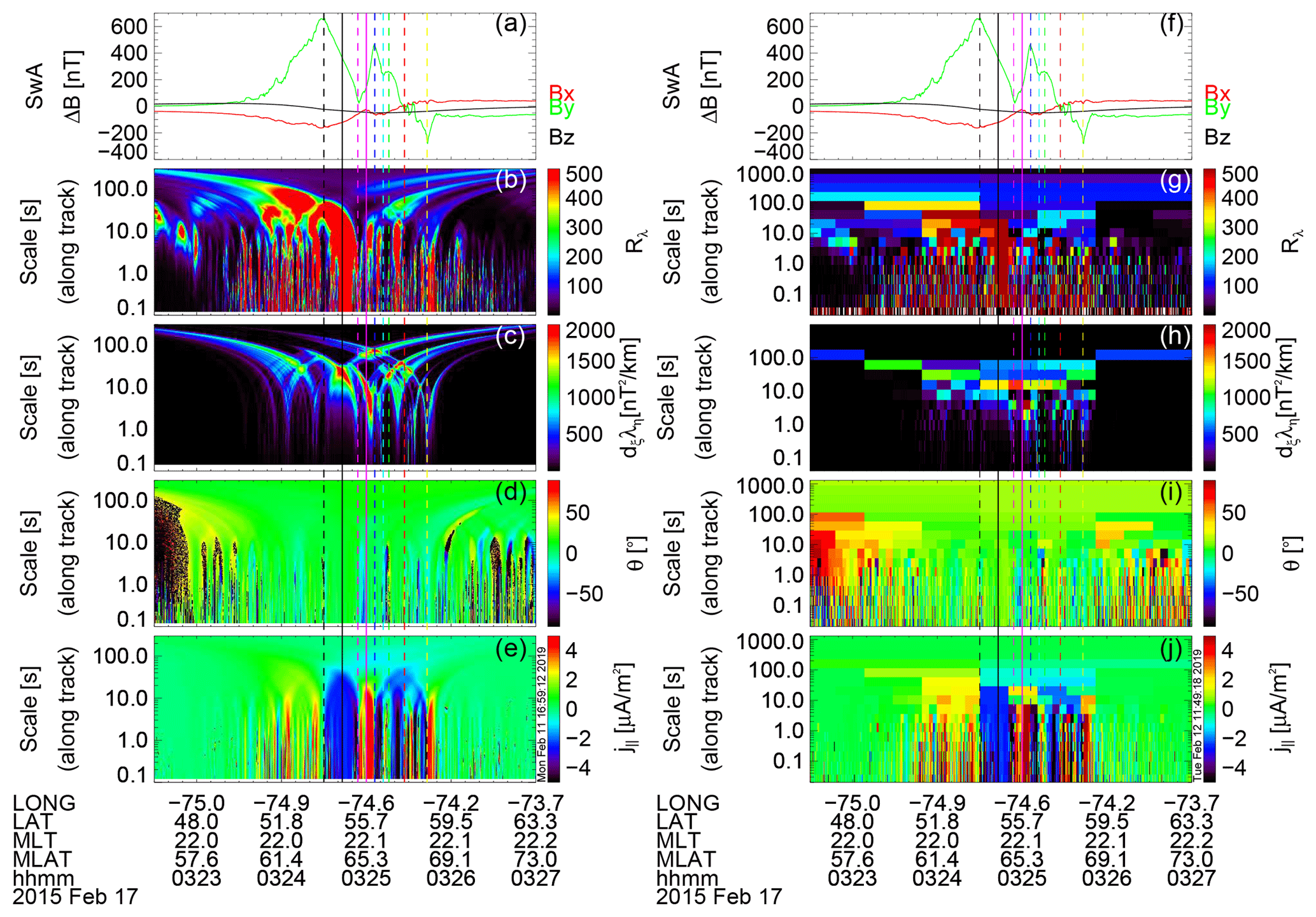
Figure 5MSMVA analysis for the linear (left) and logarithmic (right) schemes. (a) Magnetic field perturbation; (b) planarity R_λ; (c) FAC location and characteristic scale ∂_ξλ_η; (d) orientation; (e) multiscale FAC density; (f)–(j) show the same quantities for the logarithmic-scale sampling. MSMVA parameters represented as a function of the along-track scale. The vertical dashed lines delimit FAC segments as shown in Fig. 4. The vertical solid lines indicate the times for which we show the sections in Fig. 6.

Download

The left part of Fig. 5 shows the results of the linear MSMVA for SwA. The planarity, shown by the R_λ scalogram (Fig. 5b), indicates regions of high planarity for several large-/small-scale FACs, e.g., U1–3 and D1–2. The scalogram of ∂_ξλ_η (Fig. 5c) shows the location and thickness of FAC structures, whereas their orientation (Fig. 5d) confirms the optically observed alignment of the normal with the northerly direction, $\mathit{\theta }\approx \mathrm{0}{}^{\circ }$. Some typical threshold values of R_λ associated with planar structures are about 10–30 (for 3-D MVA). Because we use the 2-D MVA (B_⟂ perturbation), R_λ shows larger values, consistent with a reduced variance. We note that the investigation of the relationship between the longitudinal extension of FACs and the R_λ ratio can actually be done by using correlation analysis of the two longitudinally separated Swarm spacecraft. One expects that R_λ will be able to provide a more quantitative indication of the FAC east–west length. This topic is considered for a future study.

Panel (e) shows the newly introduced linear multiscale FAC density (Sect. 2). We can easily see the different regions of upward and downward currents at different scales, e.g., large-scale R1/R2 FACs at scales larger than 100 s, better visible in the logarithmic sampling, and smaller-scale FACs (U1-3, D1-2) at lower values, better visible in the linear sampling. The negative/positive large-scale trend is associated with upward/downward FACs, consistent with the statistical FAC model (Iijima and Potemra, 1976b) around 22:00 MLT. An alternative identification of the large-scale FACs is done by Wu et al. (2017) directly with single-spacecraft FAC density by computing the ratio of the upward and downward currents to the total current.

These representations provide a new visualization of the FAC currents dependent on scale. The linear scanning of FACs uses a large number of scales sampled at high resolution. As already mentioned, one limitation in the integrated FAC estimate for this approach is that it does not rely on an orthogonal basis and thus the integration over scales does not provide a global FAC density similar to the single- and dual-spacecraft FD methods. In order to partially improve the analysis towards an orthogonal basis we computed the same parameters also for the logarithmic scanning procedure (Sect. 2). Panels (f)–(j) show MSMVA quantities for the logarithmic scanning. In this case, the scale range extends to higher values (∼1000 s = 16.6 min) and from about 200 s (1381 km mapped to ionosphere) up one can see a close to zero net current. While the resolution is not suitable to obtain precise information on the scale dependence of these quantities, the results are in good qualitative agreement with the linear scanning.

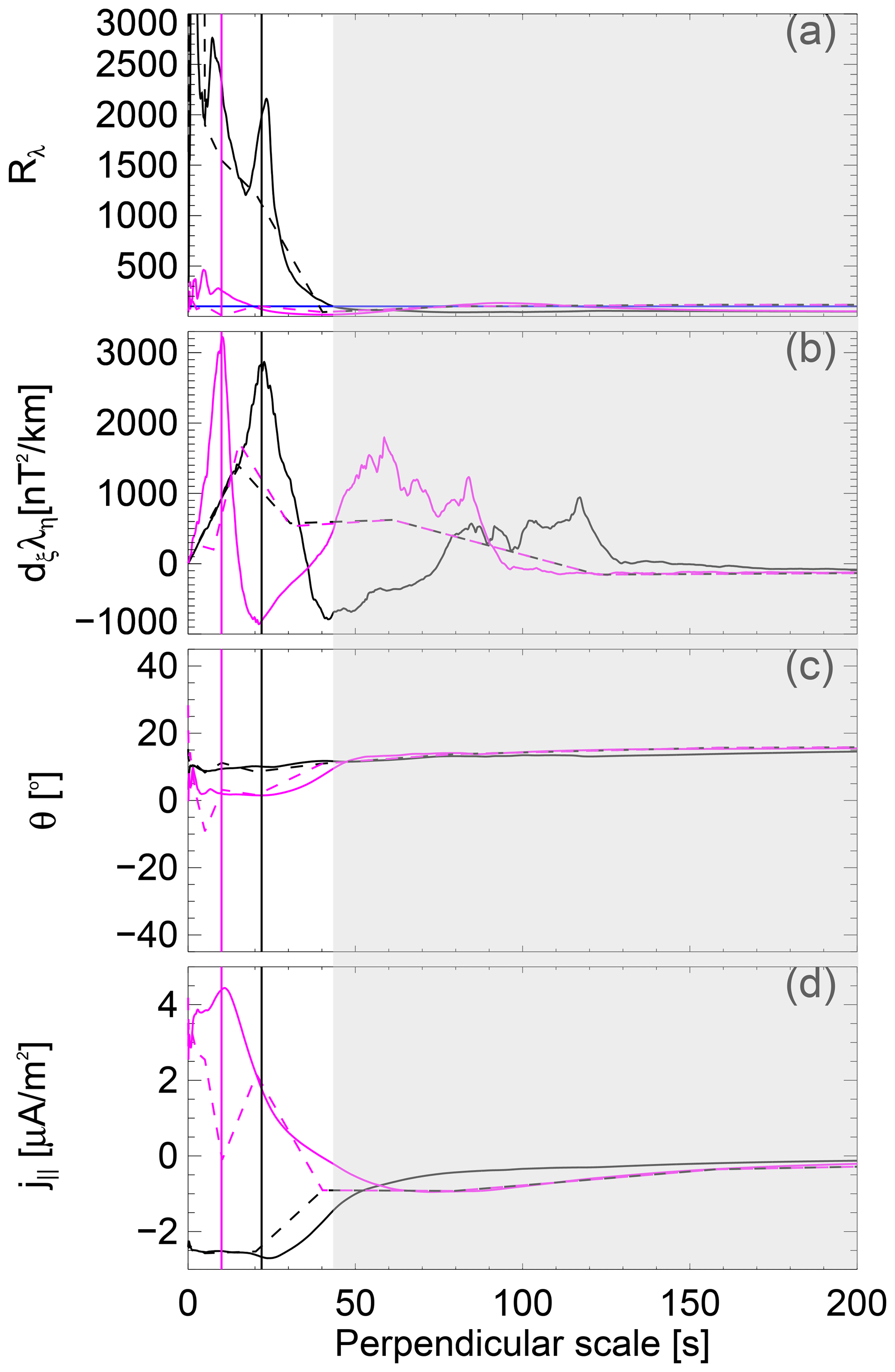
Figure 6Sections in the MSMVA scalograms showing the dependence of the parameters as a function of the perpendicular scale (scale corrected). (a) R_λ; (b) ∂_ξλ_η; (c) θ; (d) j_∥. Solid/dashed lines indicate the profiles for the linear-/logarithmic-scale sampling scheme. The profiles are taken in the middle of the upward and downward FACs located at 03:24:43 and 03:25:00, respectively. These times are indicated by the vertical solid lines in Fig. 5 (same color code). The vertical black/magenta lines indicate the scales of these FAC elements as identified by ∂_ξλ_η. The horizontal blue line in (a) indicates a reference level, R_λ=100, discussed in the text. The marked gray area indicates the region where R_λ<100 for the selected sections.

Download

Figure 6 shows a more quantitative comparison of the MSMVA quantities, including FAC density given by the two scanning schemes. We show the scale dependence of R_λ, ∂_ξλ_η, θ, and j_∥ at the center of the FACs as identified by ∂_ξλ_η and indicated by the solid lines in Fig. 5. The selected times are t_U1= 03:24:43 and t_D1= 03:25:00, associated with U1 and D1, respectively. All quantities are represented as a function of the corrected scale, similarly to the synthetic data (Sect. 3) and neglecting the small inclination of the Swarm trajectory with respect to the x axis (direction pointing north). One can see that all quantities have local maxima around the same scale, indicated by the vertical dashed lines at 22 and 10 s for U1 and D1, respectively. These scales correspond to about 153 and 70 km in the ionosphere. R_λ shows a high planarity at these two scales, with values larger than 100 (threshold indicated by the horizontal blue line) for both FACs in the linear sampling. The logarithmic sampling shows smaller values, with a smoothing of the linear profile and values below the threshold for D1. For the logarithmic sampling ∂_ξλ_η shows a similar scale, 16 s (110 km at ionosphere), for both U1 and D1 FACs. The orientation is consistent for both linear and logarithmic sampling, θ=10^∘ for U1 and ∼2^∘ for D1. In the case of rather uniform FAC density (U1 and D1) we observe that the maxima of ∂_ξλ_η are almost aligned with local maxima in R_λ, which is consistent with the intuitive expectation that the planarity of a sheet-like FAC structure maximizes around the scale (thickness) of the sheet.

The FAC density at U1 and D1 is around −2.7 and 4.5 µA m⁻², respectively, for the linear sampling. In the case of logarithmic sampling, j_∥ (dashed lines in panel d) shows roughly similar results where the respective scales are properly sampled. We have agreement for U1 ($\sim -\mathrm{2.5}$ µA m⁻²) and a close to zero FAC density for D1. The zero estimate of the current for D1 in the logarithmic scanning is caused by imperfect centering at that scale with respect to the linear scanning. Most likely, it is evaluated between U1 and D1, where we have a compensation of the currents from the two FACs. The profile of j_∥ for D1 corresponds to the same scale, but it is evaluated at a different point with respect to t_D1. For the logarithmic scheme, precise comparison with the linear scheme can be obtained at the centers of the sampled intervals (Fig. 5j).

Due to the high planarity and relatively large thickness, U1 and D1 structures satisfy the assumptions of the single- and dual-spacecraft methods. The FAC density in the single-spacecraft approximation (panel d in Fig. 4) at t_U1 and t_D1 shows values of −2.37 and 4.02 µA m⁻², respectively, whereas the dual-spacecraft FAC estimate indicates values of −3.21 and 2.58 µA m⁻². These values indicate deviations of the local FAC density (linear) with respect to single-spacecraft FAC ($\mathrm{100}\cdot (j_{\parallel }^{\mathrm{MSMVA}}-j_{\parallel }^{\mathrm{sc}})/j_{\parallel }^{\mathrm{sc}}$) of about 14 % and 12 % for U1 and D1, respectively. The same estimates with respect to the dual-spacecraft FAC density are −15 % and −74 %. The main characteristics of U1 and D1 FACs, including the percentage differences between the FAC density estimates (multiscale, single-, and dual-spacecraft) are summarized in Table 1. The deviation of the local FAC with respect to the dual-spacecraft FAC density is consistent with the scale information, low/high deviation for large/small-scale FACs. While U1 scale (153 km) is close to the resolution limit (150 km) of the dual-spacecraft method, the scale of D1 is below this limit. Considering the uncertainties in the scale definition and estimate of the FAC density, we consider that the differences between the local FAC density and the single-spacecraft estimate (<15 %) indicate a good agreement.

Table 1Comparison of the FAC estimates for 17 February  2017. Columns show perpendicular scale, FAC inclination, FAC density from multiscale, single- and dual-spacecraft, and the relative differences between the FAC densities.

Download Print Version | Download XLSX

Through the continuous and multiscale MSMVA analysis we identify the discrete FAC elements associated with the measured magnetic field perturbation. The sections in the MSMVA scalograms quantify how much current one has at the respective FAC structure. The results show the difficulty of dealing at the same time with a meaningful local FAC density estimate at a given scale and the need for orthogonality in the MSMVA basis functions. While FAC density is correctly inferred locally, one cannot compute a global FAC density estimate by integration over scales due to the lack of orthogonality of the basis functions. The sections shown in Fig. 6 were selected around the local maxima of ∂_ξλ_η. The sharp maxima of ∂_ξλ_η for U1 and D1 agree with structures of constant current densities (Bunescu et al., 2015), also expected from the ΔB profile. The gray shaded area in Fig. 6 shows the range of scales for which R_λ is below an arbitrary reference level of 100. This indicates the possibility of cleaning MSMVA quantities based on the planarity level. Such an option is needed for a multi-event or statistical study on the scale dependence of FAC characteristics. Overall, the sections into the MSMVA scalograms indicate consistent results, since all quantities show roughly the same scale. One can also note that the linear scheme is better suited for scale analysis.

A comparison of the regular single-satellite FAC density with the MVA-corrected FAC density product, albeit without scale dependence, is also included in Gillies et al. (2015) for nine events of pulsating aurora. Gillies et al. (2015) found consistent results between the two estimates at the edges of the patches associated with $R_{\mathit{\lambda }}={\mathit{\lambda }}_{\mathrm{int}}/{\mathit{\lambda }}_{\min }>\mathrm{10}$ for which the infinite FAC sheet approximation was considered valid, whereas within the patch the criterion R_λ>10 was fulfilled for only five out of nine events.

The multiscale FAC density benefits from the orientation computed at each scale. For the case of east–west aligned FACs, this may have less influence, even though one cannot exclude the possibility that some FAC elements, in a certain range of scales, are not east–west aligned. The more so, one can expect differences for events of inclined FACs. Typically, the quiet aurora during the growth phase has the normal direction aligned with the northerly direction. By using the multiscale approach one can check whether this is true also for the embedded small-scale FACs. During the onset, expansion, or early recovery phase the aurora is typically dominated by 2-D forms, possibly including locally planar small-scale FACs. By using the multiscale estimates, one can better quantify the FACs with respect to their orientation as a function of scale. This might help to quantify whether the embedded FACs are forced to have the same orientation as the large-scale FACs and, further on, possible relationships between the respective mechanisms. The FAC density scalogram combined with the other information of MSMVA provides a more intuitive and visual representation that can help to search the data for particular information.

4.3 Inclined auroral structures

This event was observed by Swarm and RANK station of the THEMIS ASI network on 15 January 2015 around 07:39 UT. The event was observed after a long quiet period, during the growth phase of a substorm with maximum ∼1 h later and, possibly, during/after pseudo-breakup activity. The AE index is ∼70 nT and DST between −5 and −8 nT. The optical frames under the spacecraft track (07:39:27–07:39:54) are shown in Fig. 7. The optical frames from the southward pass of Swarm over RANK were not included since the structures are not clearly visible. ΔB shown below indicates locally planar FACs also in this region. Overall, the optical data show a larger-scale structure inclined with respect to the east–west direction (the angle between the normal to the FAC and north is about −20^∘). Embedded smaller-scale FACs with a limited east–west extent are visible in the central region at slightly different orientations. In the center of the RANK FoV SwA/SwC are crossing different structures. The two planar FACs are about parallel, as shown also by the magnetic field data below. The RANK keogram (Fig. 8a) shows a patchy character related to the structuring of aurora. While not detailed here, a more consistent display of the time evolution of aurora can be obtained through the satellite-aligned keograms SAK (Gillies et al., 2015) obtained by stacking in time the line of pixels along the spacecraft trajectory. This is particularly useful for small-scale structures, e.g., pulsating auroral patches (Gillies et al., 2015).

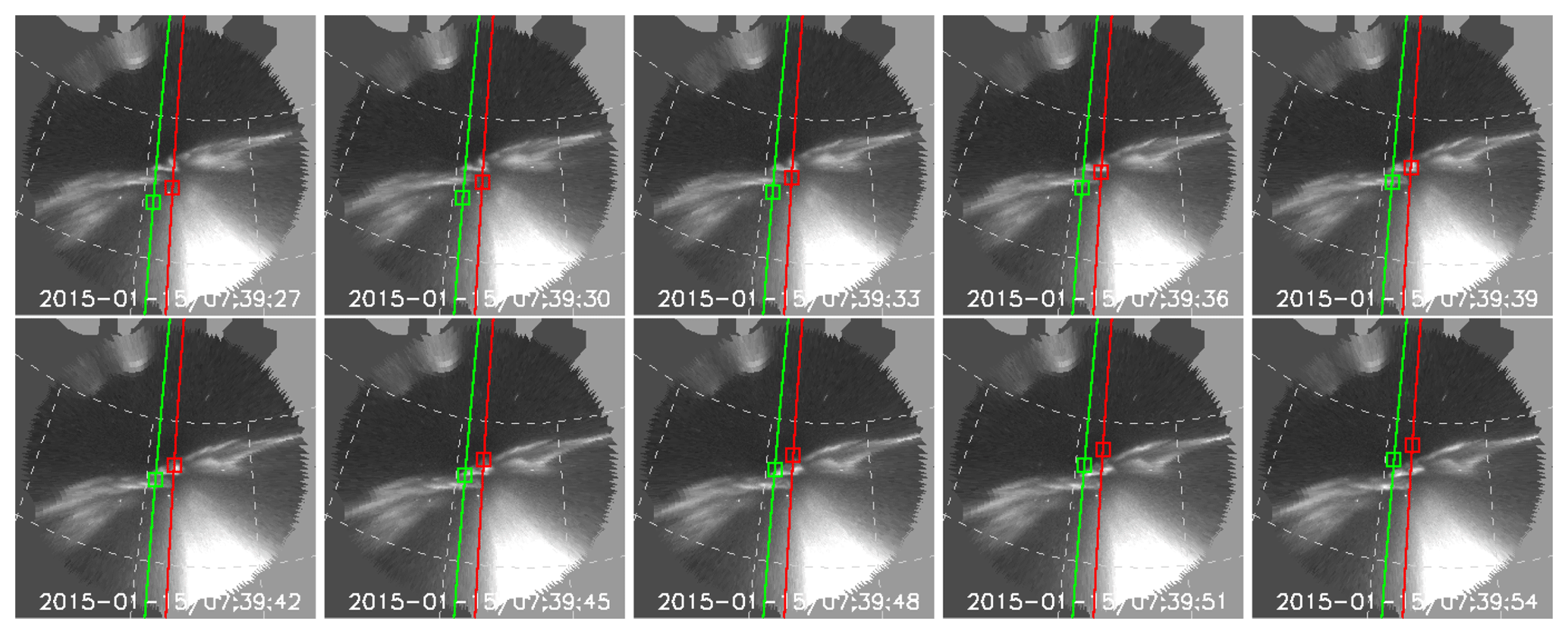
Figure 7Mapped optical frames in geographic coordinates from RANK station. The tracks show the ionospheric projection of SwA (green) and SwC (red). At the time of the frame the spacecraft mapped position is shown by the square symbols. The time is overplotted on each frame and covers the interval from 07:39:27 to 07:39:54.

Download

Figure 8 shows Swarm measurements of ΔB, FAC density estimates, and ΔB hodogram. Consistent with the inclination of the FAC structures, we have a stronger northward B_x component of B_⟂ up to about 100 nT. One can expect that the calculation of the typical single-spacecraft FAC density that neglects B_x component would lead to an underestimation of j_∥. ΔB (Fig. 8b and c) indicate similar FAC structures observed by SwA and SwC. Without optical data one could think that the two spacecraft are crossing the same structures, because of the similarity of B signatures, possibly with same dynamics considering that B_x component is varying. The L2 single-satellite FAC density (1 s resolution), shown in panel (d), indicates an oscillatory signature, associated with crossing a sequence of upward and downward FACs. The oscillations are also shown by the two-spacecraft FD estimate (black line). One can expect that the two-spacecraft estimate will rather not be suitable for describing the internal structure observed optically for this event because the assumption of uniformity over the quad surface is likely not satisfied well, e.g., in the central region of RANK's FoV. The two-satellite method can average over different structures. In this respect, the scanning of FACs by using MSMVA can help to visualize and characterize the observations of geometry (R_λ) and orientation (θ). For completeness, panel (e) shows the hodogram for this event. The intervals and the color code assignment is the same as for the previous event. Moving towards higher latitudes, SwA is crossing successively several upward and downward FAC segments colored by black, magenta, blue, cyan, green, yellow, red, and black in the hodogram. We label the delimited upward FACs by U1–U4 and the downward regions by D1–D4. The magenta interval shows also a substructure of three FACs. The difference with respect to the previous case is that for this event we have a more complex current system with embedded mesoscale FACs superposed mainly on the large-scale upward FAC, consistent with the optical data.

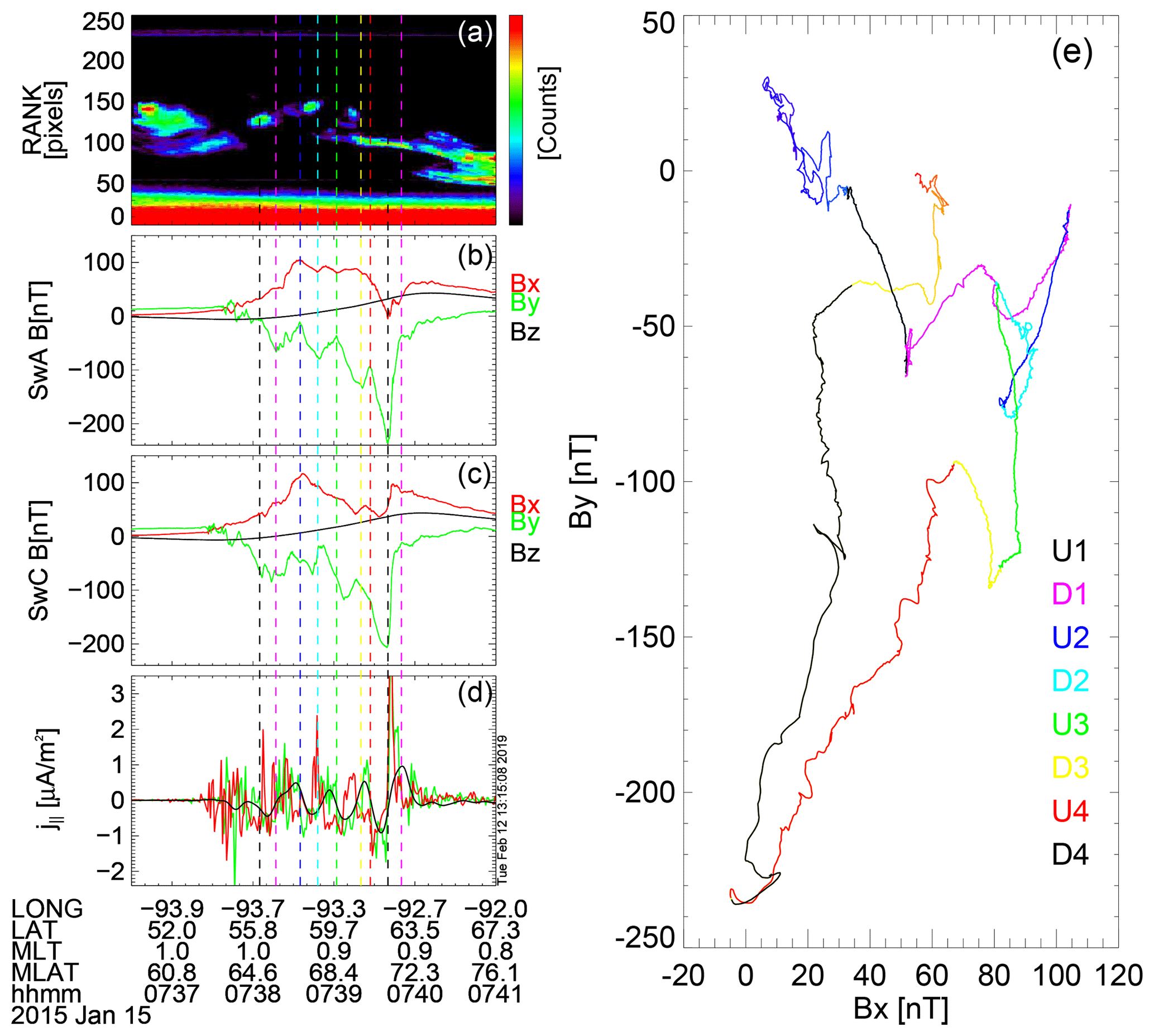
Figure 8Same panels as in Fig. 4. We note that some of the delimited FACs also have an internal structure, e.g., first magenta interval labeled D1.

Download

Figure 9 shows the results of the multiscale analysis for SwA. The left/right plots show the comparison of linear/logarithmic scanning schemes. R_λ (Fig. 9b) shows high values for some of the mesoscale FAC structures in the southern part of the RANK location, not well visible optically. Higher values are also associated with the crossing of the FAC system in the center of the FoV. By comparing R_λ values with the previous event we observe a decrease in planarity level by half, consistent with the sub-structuring of aurora, finite east–west aligned FACs. We also observe the alternation of high- and low-planarity regions, well correlated with regions of upward and downward currents, respectively, in the mesoscale range. High planarity at small-scale FACs is embedded also in the downward current regions. The scalogram of ∂_ξλ_η (Fig. 9c) shows high intensity for the U4 and D4 regions. The scale associated with the U4 and D4 regions is around 10 s (70 km). The orientation (Fig. 9d and i) at these scales is $\sim -\mathrm{20}$ and ∼0^∘, respectively, qualitatively consistent with the optical data. The j_∥ scalograms (Fig. 9e and j) show well the embedded regions of upward and downward directed currents. One can zoom into this display to get information at smaller scales, e.g., the region adjacent to the equatorward part of the track.

Figure 9Same panels as in Fig. 5. The vertical solid lines indicate the center times of U2 (blue), U3 (green), and U4 (red) FACs for which we show the sections in Fig. 10.

Download

Similar to the previous event, in Fig. 10 we show sections into MSMVA scalograms to infer quantitative estimates of the scales and current densities for a few selected FAC elements. The times of the sections are 07:38:41 (blue), 07:39:09 (green), and 07:39:33 (red). These times, indicated by the solid lines in Fig. 9, are all located in upward current regions, U2, U3, and U4, intervals. As before, for all profiles we show the dependence on the corrected scale (taking into account the inclination). R_λ shows values larger than 100 for all selected upward FACs. The maxima of ∂_ξλ_η at larger scales correspond to remote FAC elements, e.g., U4 and D4 (see Fig. 9). We note the slight shift between R_λ local maxima and the maxima of ∂_ξλ_η and j_∥. We have good agreement between the linear and logarithmic sampling for the identification of the scale for U2 and U4, whereas U3 is not properly sampled by the logarithmic scheme. We note scales of ∼12–14 s (84–98 km ionospheric scale) for the three FACs. The scale dependence at these sections shows again clearly that a masking procedure based on R_λ would be effective in removing the features associated with remote FACs crossed earlier or later. The orientation (panel c) shows an inclination of about −18^∘ for U2 (blue), 4.5^∘ for U3 (green) and −25^∘ for U4 (red), with roughly similar values in the two sampling schemes and consistent with the optical data.

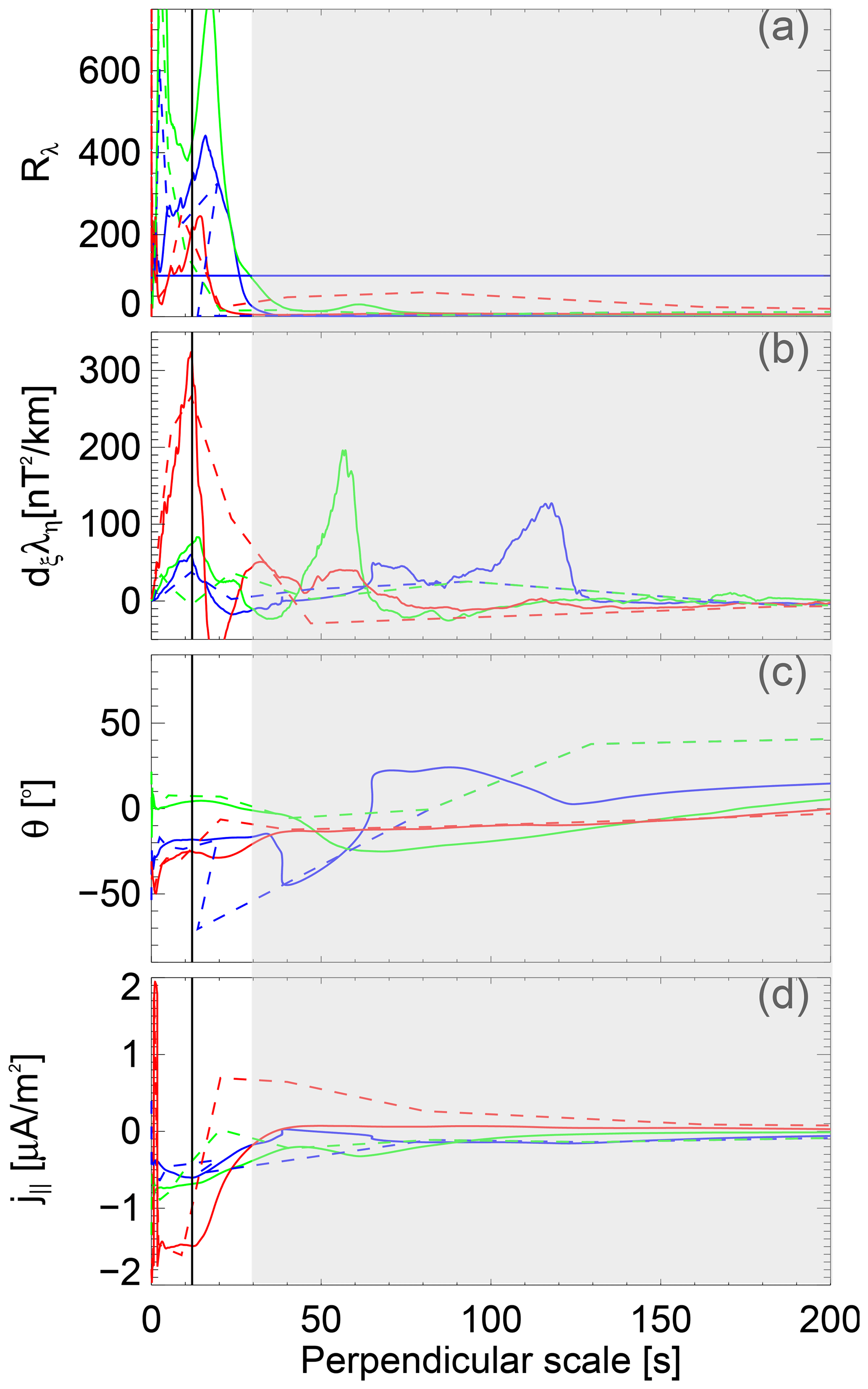
Figure 10Same panels as in Fig. 6. Solid/dashed lines indicate the profiles for the linear-/logarithmic-scale sampling scheme. The profiles are taken in the middle of the upward FACs located at 07:38:41 (blue), 07:39:09 (green), and 07:39:33 (red). These times are indicated by the vertical solid lines in Fig. 9.

Download

The values of the FAC density at these FAC segments are about −0.6 µA m⁻² for U2, −0.67 µA m⁻² for U3, and −1.49 µA m⁻² for U4 in the linear sampling. Roughly similar currents are obtained in the logarithmic sampling. The FAC density given by the single-spacecraft L2 estimate (Fig. 8) for U2, U3, and U4 is −0.23, −0.58, and −0.66 µA m⁻², whereas the dual-spacecraft FAC estimate is −0.35, −0.52, and −0.87 µA m⁻², respectively. For U2, U3, and U4 we have deviations of the local multiscale FAC density of 161 %, 15 %, and 126 % with respect to the single-spacecraft L2 estimate.

The L2 single-spacecraft FAC product and the MSMVA analysis provide estimates of the FAC density at different resolutions, are based on a slightly different computation procedure, and address the scale aspect in a different way. The L2 single-spacecraft FAC density is provided at 1 s resolution and thus enables a characterization of the current at scales larger than or equal to 1 s and typically takes into account only the east–west component of ΔB (B_y). MSMVA provides the FAC density scalogram which is based on the magnetic field perturbation in the FAC's tangential direction (B_η).

MSMVA FAC estimates, selected based on ∂_ξλ_η, correspond to the overall (average) current at the mesoscale U2–U4 FACs. When simply compared with the instantaneous values of the L2 single-spacecraft FAC density, the differences are significant (e.g., U2 and U4) due to the mismatch of the compared scales. In order to properly compare the FAC estimates, they should correspond to similar scales. Thus, we also computed an estimate of the current at a scale similar to the U2 and U4 thickness by simply smoothing the L2 single-spacecraft current using a boxcar running average of 12 s width. Figure 11 shows ΔB and FAC density estimates from SwA. We notice that most of the mesoscale FACs (including U2 and U4) have an internal structure. For both the U2 and U4 regions we have embedded perturbations visible through the slope change in ΔB inside the respective intervals (panel a). Panel (b) shows the L2 single-spacecraft FAC (green), the L2 dual-spacecraft product (black), and the average L2 single-spacecraft FAC density (red) estimated by using the 12 s boxcar average window on the L2 single-spacecraft FAC density. The internal structure provides distinct peaks in the L2 single-spacecraft FAC product which are not visible in the average and dual-spacecraft current estimates. The comparison of MSMVA FAC density with the average L2 single-spacecraft current (see Table 2) leads to a decrease in the relative percentage differences to about ∼8 %–46 % for the selected FACs and thus confirms that the initially larger differences are due to the comparison of mesoscale FAC currents with currents associated with the internal structure of the respective FACs. Differences might also be related to the fact that the used smoothing window corresponds to an along-track scale, whereas the scales inferred from MSMVA are perpendicular scales. The small difference between the local multiscale FAC and the single-spacecraft estimate for U3 is consistent with the east–west alignment of this structure (θ<5^∘). The remaining deviations for U2 and U4 are presumably also related to the neglect of the orientation, and contribution from B_x, in the computation of the single-spacecraft FD FAC estimate. A further inclusion of the orientation in the average L2 single-spacecraft FAC product would probably make the agreement with the MSMVA result even better.

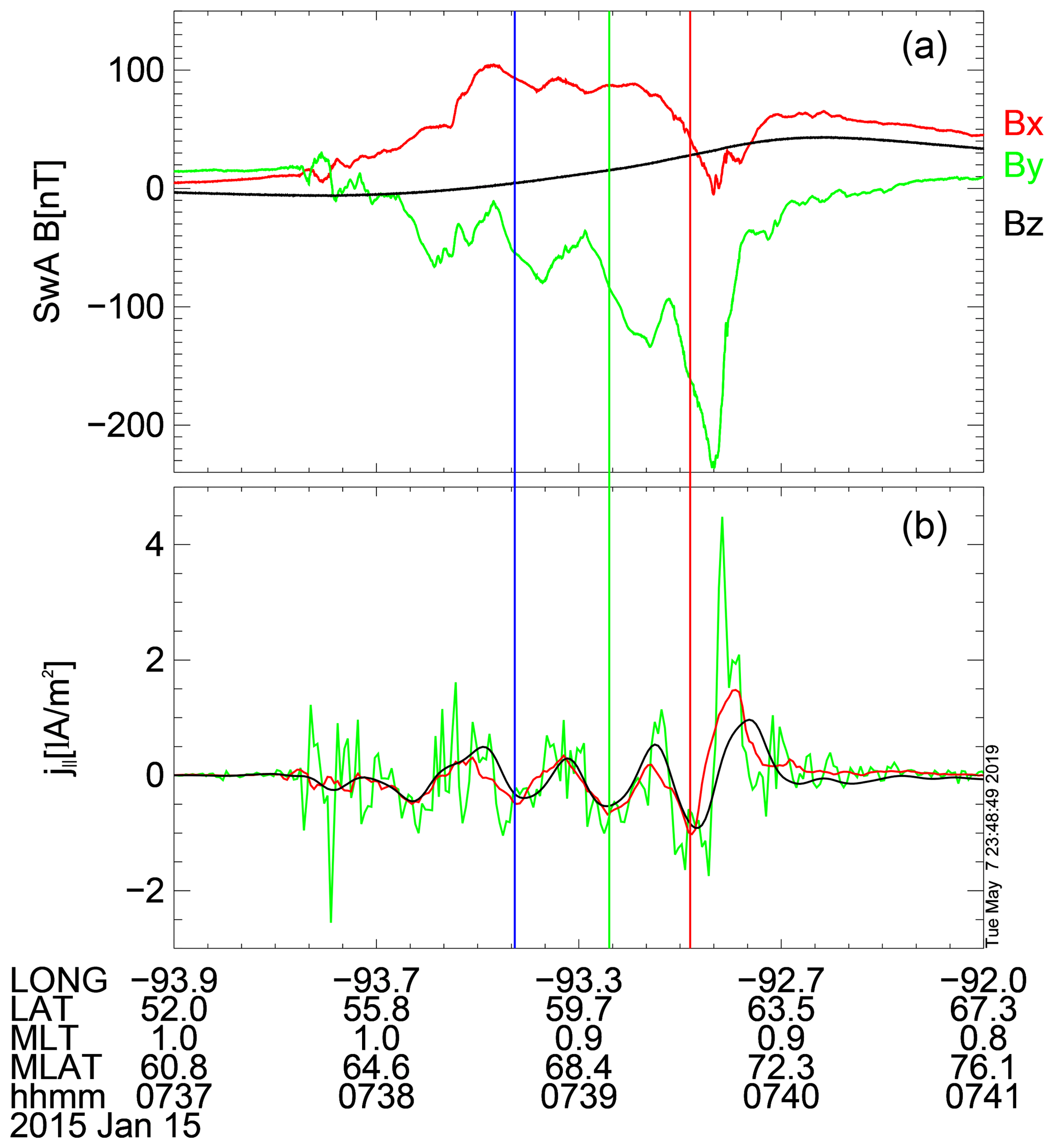
Figure 11(a) ΔB from SwA; (b) FAC density estimates, L2 single-spacecraft (green), L2 dual-spacecraft (black), average L2 single-spacecraft (red).

Download

Comparison of the local multiscale FAC density with the dual-spacecraft estimate gives 71 %, 29 %, and 71 % for the three FACs. Thus, we have again a lower difference for U3 and higher for U2 and U4. The percentages for U2 and U4 are still smaller than when comparing with the single-spacecraft estimates. Part of the differences is probably related to the resolution limit of the dual-spacecraft FAC estimates, larger than our scale of ∼83 km. The comparison between the FAC density estimates is summarized in Table 2.

Table 2Comparison of the FAC estimates for 15 January 2015 (same format as Table 1). This table shows additionally the average L2 single-sc FAC density (at 12 s scale) and the percentage deviation obtained by comparison with the MSMVA estimate. All FAC density estimates are given in µA m⁻², similar to Table 1.

Download Print Version | Download XLSX

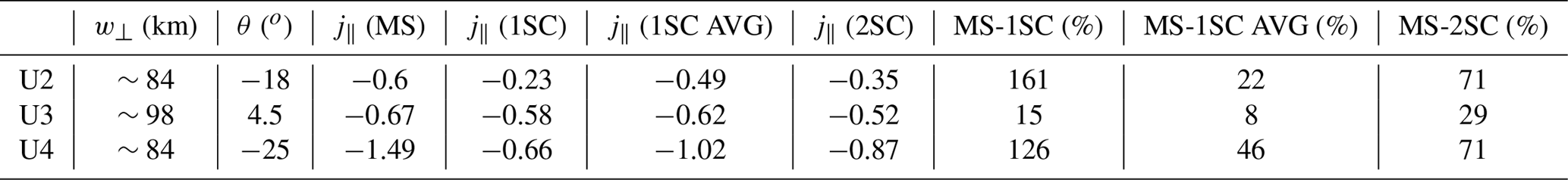
Both the linear and logarithmic samplings provide consistent information. We have similar results for the orientation and the local FAC density, whereas the scale identification can sometimes be missed in the logarithmic sampling (e.g., U3) due to the limitations of this scanning by non-overlapping intervals. This event indicates that care is needed when designing an automatic procedure for the analysis of FACs on a statistical basis. The two-spacecraft methods can average over different structures; moreover, some assumptions of the methods are possibly not fulfilled.

4.4 Small-scale auroral observations embedded in a large-scale current

The relation between multiple arc systems and their FAC signatures was addressed recently by Wu et al. (2017) based on Swarm/THEMIS ASI observations. Wu et al. (2017) selected events with clearly identifiable stable arcs and separated the observations into two categories, unipolar (multiple arcs embedded in a single large upward FAC) and multipolar events (a collection of multiple arcs and related pairs of upward and downward FACs). Arcs associated with multipolar FAC events were found to be broader and more separated than those associated with unipolar FAC events. In this section we perform MSMVA analysis for a unipolar event investigated by Wu et al. (2017).

The event occurred on 27 September 2014 around 06:00 UT, in the evening sector (∼22 MLT) and was observed simultaneously by Swarm and FSMI ASI in Canada. The event was observed during a very active period, with multiple substorms and an average AE of ∼500 nT over the hours around the event. The AE index is ∼550 and DST = −23 nT.

The mapped optical frames and the superposed spacecraft tracks, shown in Fig. 12, indicate the crossing towards the Equator of a thick auroral structure (∼ 05:59:48–06:00:00 = 12 s) followed by some small-scale less intense arcs and an intense structure around 06:00:09–06:00:12. Since the crossing is near the edge of the ASI's FoV, in the following we do not attempt to make a one-to-one matching between the optical observations and ΔB or FAC signatures.

Figure 12Mapped optical frames in geographic coordinates from FSMI station. The tracks show the ionospheric projection of SwA (green) and SwC (red). At the time of the frame the spacecraft mapped position is shown by the square symbols. The time is overplotted on each frame and covers the interval from 05:59:39 to 06:00:12.

Download

The MLT location of the event and the optical data indicate the crossing near the Harang discontinuity region. Following the Swarm track (north to south), the statistical model of FACs (Iijima and Potemra, 1976b) indicates the crossing of the large-scale downward, upward, and downward FACs. Figure 13 shows again ΔB, FAC density, and the ΔB hodogram. ΔB for both SwA and SwC (Fig. 13b and c) show the three large-scale FACs with embedded smaller-scale structures. The FAC density estimates are shown in panel (d). We note the high fluctuation level in the single-spacecraft estimates caused by small-scale FACs. The two-spacecraft method shows likewise the large-scale FACs and does not capture small-scale currents, which are dynamic, since the related signatures on the two spacecraft, separated by ∼10 s in latitude, are different. The small-scale features are captured by the single-satellite FAC estimates, but it is difficult to quantify their characteristics based only on this information. Comparison of ΔB from SwA and SwC shows more clearly small-scale perturbations on SwC in the green interval. Thus, in the following we perform MSMVA analysis on SwC.

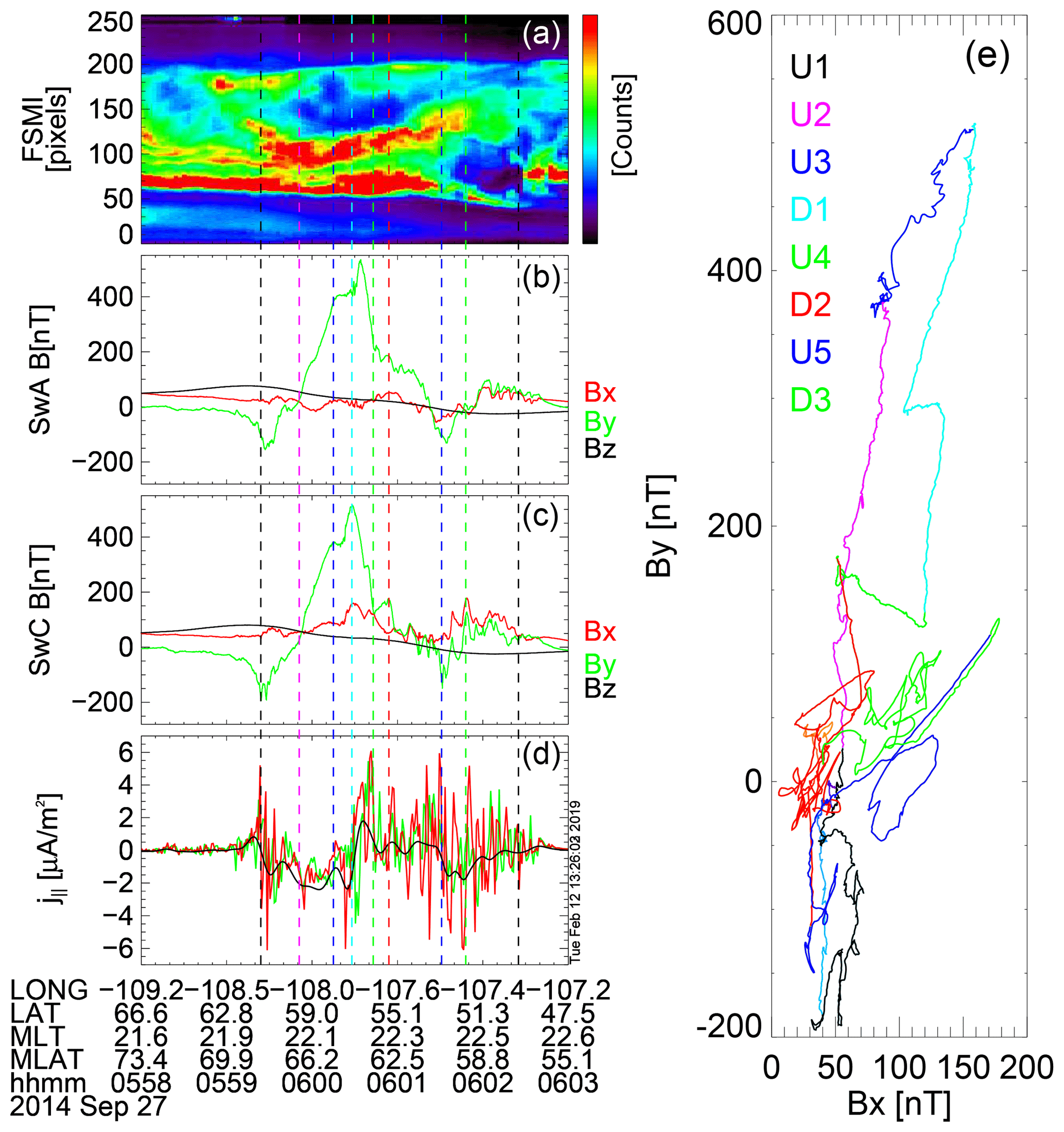
Figure 13Same panels as in Fig. 4. The vertical lines indicate individual FACs, e.g., first black, magenta, and blue intervals, or larger intervals with small-scale FAC signatures, e.g., red, second blue, or second green intervals.

Download

The hodogram (panel e) shows the typical characteristics observed for the previous events. The interval color is given by the color of the left vertical dashed line, which for this case is related to ΔB from SwC. The prevalence of ΔB_y indicates a close alignment of the arcs with the east–west direction. We note that in this case the relationship between the FAC direction and the slope of ΔB is opposite with respect to the other events, consistent with the equatorward crossing of Swarm. The U/D labels are associated with positive/negative slope of ΔB and negative/positive j_∥ (see Sect. 2.2, Eqs. 4 and 5). Embedded small-scale FACs segments are seen in the red (D2) and second green (D3) intervals, which also show a rotation in the hodogram specific to wave activity.

Figure 14Same panels as in Fig. 5. The vertical dashed lines indicate the FAC segments or intervals of small-scale FACs. The vertical solid lines indicate the central times of small-scale downward (black) and upward (green) FAC elements for which we show the sections in Fig. 15.

Download

Figure 14 shows the results of the linear and logarithmic FAC scanning. The intensity of the scalograms for the linear scheme is also shown in logarithmic scale to emphasize the small-scale FACs. The highly planar FACs at small-scales are confirmed by R_λ scalogram (Fig. 14b and g), consistent with the hodogram. The general description from the previous events applies also here. In the following, we select and analyze in more detail a few small-scale FACs, indicated by the solid vertical lines. The black/green color indicates downward/upward FACs. Here we do not distinguish between these small-scale downward FACs and just infer a range of the parameters. Figure 15 shows the sections in the MSMVA scalograms at the respective times. We observe again that remote FACs have a smaller impact on R_λ as compared to ∂_ξλ_η. All selected small-scale FACs show a high degree of planarity. The dependence of ∂_ξλ_η on scale indicates a range of scales between 1.8 (12.4 km) and 4 s (27.6 km) (shown by the vertical red lines) for the selected FACs. The orientation shows values from $\sim -\mathrm{40}$ to ∼10^∘. The FAC density has values of about −7.5 µA m⁻² for the upward region (green) and between 4 and 6 µA m⁻² for the four downward FACs. For this event we can make just a qualitative comparison with the single-spacecraft FAC estimates since the scales are well below the resolution of the dual-spacecraft estimate. The single-spacecraft FAC density is −4.24 µA m⁻² for the upward FAC and between 3.84 and 6.08 µA m⁻² for the downward FACs. Thus, we have roughly similar values for downward FACs with small inclination (<10^∘) and higher deviations for the highly inclined FACs, e.g., upward FAC element. The detailed analysis (not shown) indicates that the selected times are associated with local maxima of the single-spacecraft FAC density and this indicates the consistency of ∂_ξλ_η information at small scales.

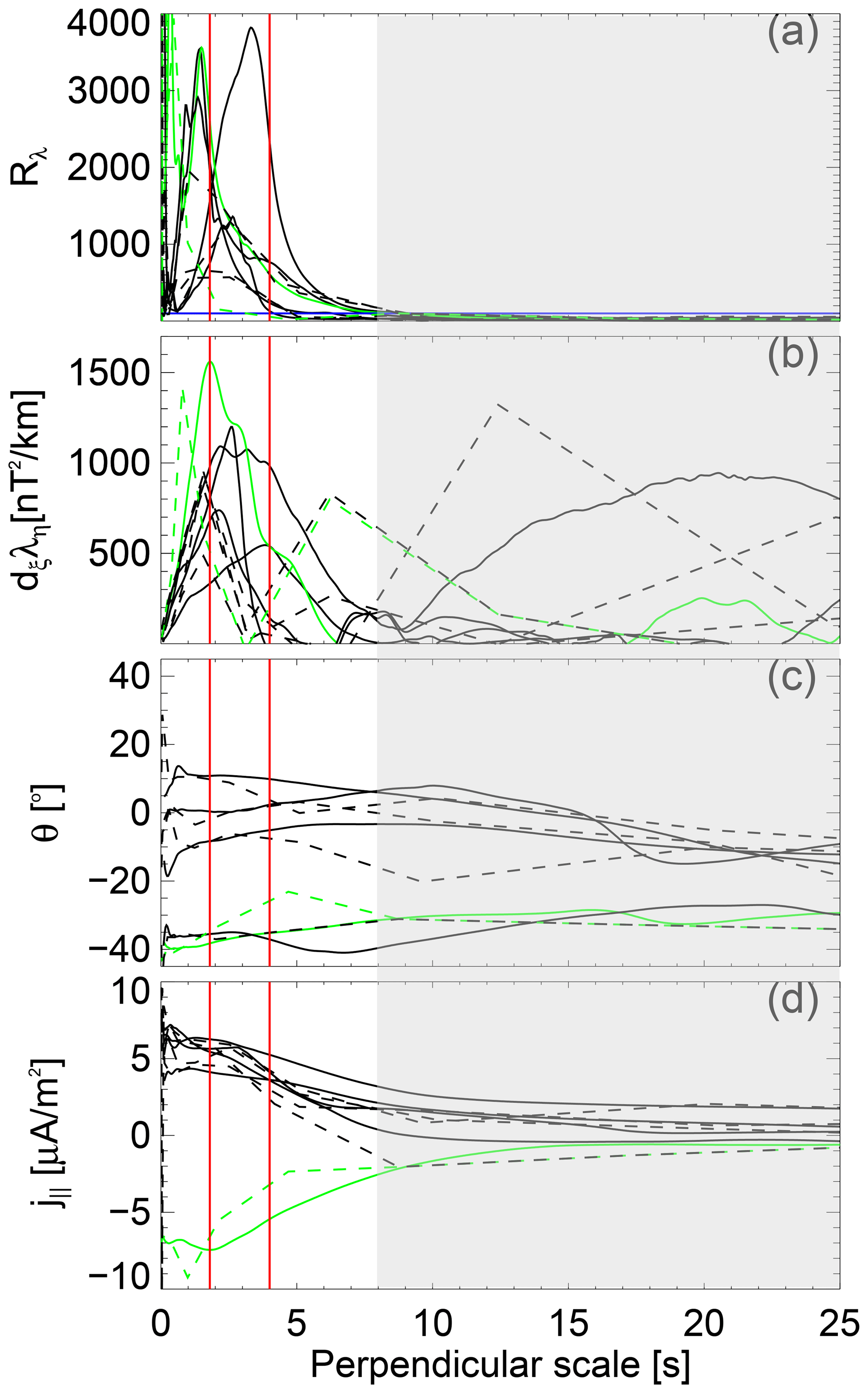
Figure 15Same panels as in Fig. 6. Solid/dashed lines indicate the profiles for the linear-/logarithmic-scale sampling scheme. The vertical red lines indicate the domain of scales identified by ∂_ξλ_η for the upward (green) and downward (black) FACs.

Download

When going to smaller scales, non-stationary effects become more important and can be characterized by using the nested MVA analysis. This procedure is implicitly included in the MSMVA technique since at each point we perform a nested MVA in the linear scanning. The standard nested MVA (Sonnerup and Scheible, 1998) is applied in 3-D and investigates the scale dependence of orientation and projections of B on the eigenvectors. In this study, we extended MSMVA analysis by the density scalogram and showed quantitative estimates of the local current density for FACs observed by Swarm.