the Creative Commons Attribution 4.0 License.
the Creative Commons Attribution 4.0 License.
 | 28 Nov 2019
Magnetic local time asymmetries in precipitating electron and proton populations with and without substorm activity
Olesya Yakovchuk
Jan Maik Wissing
The magnetic local time (MLT) dependence of electron (0.15–300 keV) and proton (0.15–6900 keV) precipitation into the atmosphere based on National Oceanic and Atmospheric Administration POES and METOP satellite data during 2001–2008 was described. Using modified APEX coordinates the influence of particle energy, substorm activity and geomagnetic disturbance on the MLT flux distribution was statistically analysed.
Some of the findings are the following.
- a.
Substorms mostly increase particle precipitation in the night sector by about factor 2–4, but can also reduce it in the day sector.
- b.
MLT dependence can be assigned to particles entering the magnetosphere at the cusp region and magnetospheric particles in combination with energy-specific drifts (in agreement with Newell et al., 2009).
- c.
MLT flux differences of up to 2 orders of magnitude have been identified inside the auroral oval during geomagnetically disturbed conditions. The novelty here is the comprehensive coverage of energy bands and the focus on asymmetry.
- d.
The maximum flux asymmetry ratio depends on particle energy, decreasing with Kp for low energetic particles and increasing with Kp for higher energy electrons, while high energy protons show a more complex dependency. While some aspects may already have been known, the quantification of the flux asymmetry sheds new light on MLT variation.
- Article
(5276 KB) - Full-text XML
- BibTeX
- EndNote


Particle precipitation is a primary link between solar activity and atmospheric chemistry. Thorne (1977) suggested a depletion of ozone in 40–80 km through production of nitric oxides by precipitation of relativistic radiation belt electrons. Ozone depletion following solar energetic particle events (mostly protons) has been observed in the same year (Heath et al., 1977). Auroral particle precipitation causes production of HOy and NOx and thus is a significant player in mesospheric and stratospheric chemistry, especially as these chemicals catalytically impact the ozone cycle (Callis et al., 1996a, b) and subsequently change the radiation budget and affect dynamics. Consequently there has been an immanent need for the description (and later on modelling) of the particle precipitation. And even though the investigation of the precipitation pattern of low energetic particles (and especially electrons) started more then 30 years ago (e.g. Hardy et al., 1985), the rising vertical extent of climate models has shifted the focus from high energetic particles to lower energies again.
The interplanetary medium is the driver of geomagnetic disturbance and may compress, deform or reconnect to the magnetosphere. Meredith et al. (2011) e.g. state that, on average, the flux of precipitating energy electrons (E>30 keV) is enhanced by a factor of about 10 during the passage of the high-speed stream (geomagnetic storm time) at all geographic longitudes. Thus geomagnetic disturbance should be considered in a description of particle precipitation.
MLT dependence is a result of charge-dependent drift directions (Allison et al., 2017) and (linked to that) opposite potentials in field-aligned Birkeland currents. The authors themselves note that the particle flux variety in different local time sectors may reach an order of magnitude, with proton precipitation dominating in evening and night sectors and electrons dominating in the morning and night (Wissing et al., 2008).
Substorms are either directly driven or/and loading processes, where energy is accumulated and released abruptly in the Earth's magnetosphere (Akasofu, 2015). The global morphology of auroral substorms was first described by Akasofu (1964) using simultaneous all-sky camera recordings from Siberia, Alaska and Canada. Later space-borne missions like e.g. the UV photometer mission on Dynamics Explorer 1 (DE-1) (Frank et al., 1981) confirmed this morphology.
Akasofu et al. (1965) also already characterized the expansion phase and the recovery phase of a substorm (a preceding growth phase was added by McPherron, 1970). Due to auroral emissions the substorms were associated with excitation and ionization by precipitating particles that have been investigated by ground-based riometers (Berkey et al., 1974) and later on by satellite missions (e.g. Fujii et al., 1994), observing intense energetic electron precipitation in or near the onset/surge region. The energy range of the precipitating particles has been defined as electrons and protons at approx. 10–100 keV with a low-energy cut-off (Birn et al., 1997). The precipitation regions depend on particle species.
The occurrence of substorms depends on the orientation of the interplanetary magnetic field. As shown in Reeves et al. (2003), these external solar wind parameters subsequently impact the magnetic field on the ground and are represented in the Auroral Electrojet (AE) index. Auroral Electrojet indices AE = AU − AL are a good proxy of the global auroral power, where AU (amplitude upper) and AL (amplitude lower) are the upper and lower components of AE, which means the largest and smallest values of the H component among 12 magnetic stations (Davis and Sugiura, 1966). AU represents the strength of the eastward electrojet, while AL represents the westward electrojet. Consequently AL seems to be the index which best corresponds to westward intensification of the auroral current, or substorm activity. Prior to substorm onset, the AL index is typically small in magnitude, with the contributing station near dawn, whereas during substorm onset, the station contributing to the lower envelope is usually in the dusk sector under the auroral expansion. However, due to the limited spatial coverage of the 12 magnetometer stations, the auroral expansion can be missed, which means that this index does not always reflect the onset (Gjerloev et al., 2004). The use of SuperMAG SML (the generalization of AL), an index derived likewise to the AL but based on all available magnetometer stations (typically more than 100) at these latitudes, considerably improves the detection of substorm onsets (Newell and Gjerloev, 2011a). Thus we use the SML index in this study to define substorm onsets.
In this study we will discuss MLT differences in particle fluxes (and precipitation) over a wide energy range and show how substorms impact this pattern.
In Sect. 2, particle data, a modified APEX coordinate system, SML and Kp binning will be introduced. Section 3 displays the application of modified APEX coordinates to the flux maps, discusses special aspects of the MLT binning and illustrates how the auroral oval is fitted. In Sect. 4 the main discussion follows and the analysis of particle fluxes at high latitudes. The results are summarized in Sect. 5.
This section describes the data sets and how the data have been processed.
2.1 Particle data
For particle data we use time series (2001–2008) of 16 s averaged electron fluxes ranging from 0.15 to 300 keV and protons from 0.15 to 6900 keV measured onboard the polar-orbiting NOAA/POES and their successor, the METOP satellites (Evans and Greer, 2006); 2001 to 2008 cover the complete declining phase of solar cycle 23 and thus include very active (sometimes extreme) to very low activity periods (Logachev et al., 2016).
In total all available data from POES 15, 16, 17, and 18 and METOP 02 have been used, except for POES 16 after 2006, as it is known that the TED data are erroneous.
All satellites have Sun-synchronous orbits at altitudes around 820 km (with ≈100 min periods of revolution) and an inclination of ≈98.5∘. The satellites have initially been placed in orbits that cross the Equator at a fixed local time either being morning–evening or day–night sectors. However, or in our case fortunately, these orbits were drifting slightly with time. Thus our long sample period and the moving five satellites allowed us to investigate the effect of local time on particle fluxes.
Information about the different channels can be found in Table 1. All particle count rates have been converted into differential flux by dividing the energy range, and a geometric factor has been applied as suggested in Evans and Greer (2006).
It is known that there is no adequate upper energy threshold of the three MEPED electron channels (Yando et al., 2011). In order to work with specific energy bands we subtracted sequent channels, resulting in the two channels mep0e1–e2 and mep0e2–e3 with the energy bounds given in Table 1.
Table 1Channels and nominal energy ranges from the POES and METOP satellites which have been used.
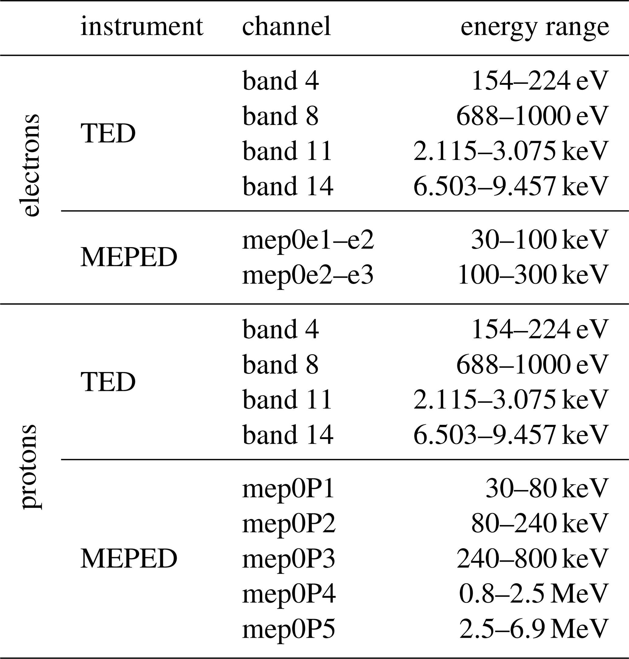
We used the 0∘ detectors only. While the TED 0∘ detector looks exactly radially outward, the MEPED 0∘ detector is slightly shifted by 9∘ to ensure a clear field of view (Evans and Greer, 2006).
The MEPED detectors have a field of view of ±15∘, while the TED detector has the following specifications according to Evans and Greer (2006): the fields of view of the electron and proton 1000–20 000 eV detector systems are 1.5∘ by 9∘, half angles. The field of view of the 50–1000 eV electron detector system is 6.7∘ by 3.3∘, half angles. The field of view of the 50–1000 eV proton detector system is 6.6∘ by 8.7∘, half angles. Opening angles of the detector in combination with the position of the satellite determine which particle populations the detector is measuring. According to Rodger et al. (2010, Fig. 1) the MEPED 0∘ detector in latitudes discussed in Sect. 4 measures particles in the bounce loss cone only.
Given that the point of view of the TED detector is almost identical to the MEPED detector and the field of view is significantly smaller, Fig. 1 in Rodger et al. (2010) can also be applied, keeping in mind that regions of overlapping particle populations will decline. Thus we can borrow the particle populations seen in the TED channels from the MEPED results. In summation: at high latitudes both detectors count precipitating particle flux, while they detect mostly trapped particles at low latitudes.
All figures in this paper show differential particle flux in (MeV m2 s sr)−1 as measured; thus, we made no assumption about a pitch angle distribution here. However, it should be noted that even if the detector is looking upward (and measuring downgoing particles at high latitudes), it does not necessarily mean that all these particles are precipitating (reaching the atmosphere). Given that some particles are mirroring above the atmosphere, a fraction of the downgoing flux is lost; thus, the magnetic flux tube is narrowing, the particle flux increases again and only in case the pitch angle distribution is isotropic is the mirrored fraction balanced by flux tube narrowing (see e.g. Bornebusch et al., 2010). And only in the case of an isotropic pitch angle distribution does it not matter for upscaling which angles of the downgoing pitch angle distribution we are measuring: an isotropic pitch angle distribution may easily be integrated over 2π to estimate the total precipitating flux over all angles.
However, it is known that anisotropic distributions occur. While an unaccelerated source population is assumed to be isotropic (as is a wave-scattered fraction of that population in the loss cone), most acceleration processes are connected with an anisotropic pitch angle distribution. Dombeck et al. (2018) list the most important ones as quasi-static-potential structures, namely an electric potential field, which may cause isotropic or anisotropic distributions, and Alfvén waves, which accelerate only particle energies that are in resonance with magnetic field waves and cause highly anisotropic distributions. Alfvén waves are responsible for electron precipitation during substorms (Newell et al., 2010). According to Newell et al. (2009) electrons are often accelerated, while ions are not.
In case of an anisotropic pitch angle distribution an estimation of the total precipitating flux is not straightforward as first a pitch angle distribution has to be assumed and second the pitch angles the detector is currently measuring have to be determined. Since the only other detector orientation on POES measures trapped particles (at high latitudes) and since trapped particles do not get lost, there is no reason to assume a smooth transition between these two particle populations. Thus we do not have a “reference” anisotropic pitch angle distribution that might be applied. Applying an isotropic pitch angle (which is often done in the literature) will put the downgoing flux on a level with precipitating flux. In the case where the paper states “particle precipitation”, this isotropic pitch angle distribution has been implicitly assumed. However, this has been made without loss of generality since the shown differential flux in that case is equal to the downgoing flux. Thus no transformation is needed.
All shown values are spatially and temporally averaged fluxes. In case a detector measures zero counts every time, it crosses a specific position, and at a certain condition this also enters the figures with zero flux (see e.g. Fig. 3, TED electron band 11, isolated substorm, −55∘ modified APEX latitude at noon). Since the detector counts are transferred into flux the MEPED channels do not recognize flux less than one count per integration interval (equivalent to 1 000 000 particles (m2 s sr)−1 divided by the channels' energy range). For the TED detector the transformation is similar, but instead of a fixed number a calibration factor has to be applied for every channel and satellite. The calibrations are given in e.g. Evans and Greer (2004).
The particle detectors suffer from various contamination effects: the MEPED electron channels are highly efficient detectors for high energetic protons. In order to avoid contaminated electron data, we excluded MEPED electrons when the omnidirectional proton channel P7 showed more than two counts (based on high-resolution 2 s data). This cuts out probably contaminated periods not only in SPEs, but also in the region of the South Atlantic Anomaly (SAA). The MEPED electron channels have been subtracted from each other, resulting in differential channels.
Note that the given energy ranges taken from Evans and Greer (2006) are nominal. Some channels suffer from degradation. This mostly holds for the MEPED proton channels and is a result of structural defects caused by the impinging particles. In the long run it causes an energy shift (to higher particle energies) since fewer electron–hole pairs are produced per deposited particle energy. Consequently the energy ranges mentioned are nominal ranges. Further details on degradation of the MEPED channels can be found in e.g. Asikainen et al. (2012).
2.2 Coordinate system
A meaningful representation of particle precipitation has high requirements for the coordinate system as follows.
- a.
The flux pattern should be invariant in time even though the magnetic field is changing (meaning moving poles, not magnetospheric distortion). This is needed for the long investigation period as well as for durability of forecasts.
- b.
The latitude of the particle flux pattern should be invariant of the longitude. Given this criterion the longitude may be replaced by local time as a second coordinate.
- c.
If the previous criterion is applied, it includes the fact that particle flux has to be recalculated. Following the footpoints of two shells with a distinct magnetic field strength, their latitudinal distance differs with longitude. Since the particle flux is measured on a fixed detector size, this has to be taken into account when removing the longitudinal dependence.
- d.
Particle measurements take place at the position of the satellite, which is about 820 km above the ground. But the effect of particle precipitation (the atmospheric ionization) is mainly located at about 110 km altitude (maximum of magnetospheric ionization; higher particle energies cause ionization further down). Consequently a coordinate system that allocates the satellite's measurement to their respective position at 110 km altitude would be helpful.
The coordinate system that allows for all named requirements is the modified APEX coordinate system (Richmond, 1995). The coordinates are variable in time using the International Geomagnetic Reference Field model magnetic field configuration, which means they also reflect the temporal movement of the poles. Richmond (1995) presents three coordinate systems which are closely connected. The quasi-dipole (QD) coordinates present the magnetic latitude and longitude on the ground (Richmond, 1995, see the f1 and f2 base vectors in Fig. 1), while the third base vector goes radially outward. The APEX coordinate system uses the same longitude, but the latitude follows the magnetic field lines as propagating (precipitating) particles do, meaning that a charged particle is always at the same latitude. The APEX latitude is defined by its footpoint at the QD latitude on the surface. In the modified APEX coordinates not the surface but an arbitrary altitude is used for the definition of the latitude, e.g. that altitude where particles cause the ionization, in our case 110 km above the ground. Thus the measurements should be mapped down on the corresponding field line until it reaches the altitude where the particle is stopped by the atmosphere (about 110 km). In all (modified) APEX systems measurements and ionization location are at the same latitude. Thus a desirable coordinate system for our work is the modified APEX system.
2.3 SML index and derived substorm onsets
The period 2001–2008 was chosen for our investigation, where all necessary data about substorms and particle fluxes are available. For the identification of substorm events, we use the technique published by Newell and Gjerloev (2011a). The substorm onset is determined by the auroral electrojet SML index, which is derived from magnetometer data obtained by the SuperMAG magnetometer network. The SuperMAG magnetometer network in the Northern Hemisphere (up to 100 stations) improves the traditional AE network (12 stations) (Newell and Gjerloev, 2011a).
Newell and Gjerloev (2011b) distinguish recurrent and isolated substorms. While recurrent substorms appear in groups with less than 82 min between their onsets, the isolated substorm onsets are separated by at least 3 h. Only the isolated substorms are used in our investigation, as this helps to avoid two or more substorms overlapping each other. Contrasting the isolated substorm periods, we also use time periods without any substorms (no-substorm period). The total number of substorm onsets for our period constitutes 15 316 events. Defining 30 min after an onset as the typical length of a substorm, we end up with 10.4 % of the whole period being generally substorm-influenced (while the rest is no-substorm). However, just 1.87 % of the whole period can be attributed to isolated substorms.
It should be noted that with this technique we are not able to separate different substorm phases nor can we distinguish different types of substorms. Independent of substorm phase, the proton aurora is displaced equatorward of the electron aurora for dusk local times, and it is poleward for dawn local times. In the onset region, however, proton and electron precipitation depends on the substorm phase and may even be co-located (Mende et al., 2003). Thus the results represent a mean substorm value.
2.4 Kp binning of particle data
The Kp index is a 3-hourly index estimating the geomagnetic activity (Bartels et al., 1939). In contrast to the AL/SML index which describes the auroral electrojet activity, the Kp index is sensitive to several current systems (e.g. the ring current) and thus describes the magnetospheric activity with a more global perspective.
The particle data have been binned into 11 partly overlapping Kp-level groups: 0–0.7, 0–1, 1–1.7, 1.3–2.3, 2–2.7, 3–3.7, 4–4.7, 5–5.7, 6–6.7, 6–9 and 7–9. As the Kp levels are not equally populated (low Kp levels occur more frequently than e.g. 6–6.7), the number of satellites is not constant, the substorms are not evenly distributed in time and the local time sectors are not evenly covered, single data points (with 1 h MLT resolution, 2∘ latitudinal resolution and the Kp binning) may contain a different amount of the 16 s averages.
Binning of particle flux strongly depends on the coordinate system. Some features are determined by the inner magnetic field and are thus co-rotating with Earth, while others are influenced by the interaction with the solar wind and according to that fixed in relation to the Sun and to the (magnetic) local time. Since we will use the modified APEX coordinates in this paper, we will have a look at how the particle flux representation differs from geographic coordinates and which aspects can be best described in the two systems.
Figure 1 shows TED proton band 11 in geographic coordinates (top row) and modified APEX 110 km coordinates (bottom row). The left column shows latitude against longitude, while the right column shows latitude against MLT. No selection according to Kp level or substorm intensity has been made, while all available data from METOP 2 and POES 15, 16, 17 and 18 for the years 2001–2008 have been included. This allows a spatial resolution of 3.75∘ longitude (or 15 min MLT). Please note that the latter figures show a reduced longitudinal resolution of 15∘ (or 1 h MLT) only to avoid statistical noise in e.g. isolated substorm periods.
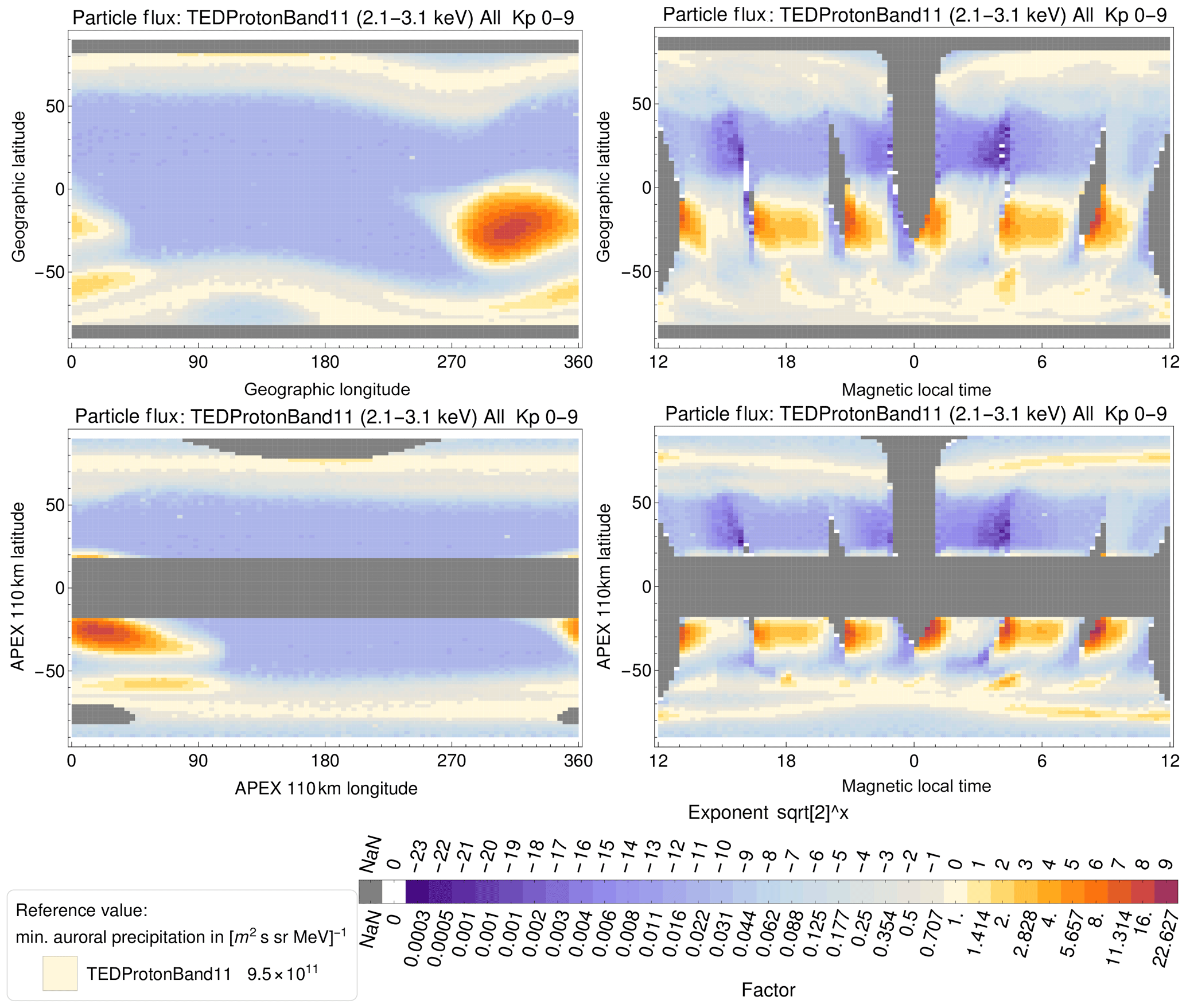
Figure 1Particle flux in TED proton band 11 in geographic and modified APEX 110 km coordinates. The colour scale marks the minimum flux in the auroral oval in beige. The neighbouring colour indicates that the flux is a factor apart (the neighbour after that a factor 2).
Most obvious in the geographic representation (Fig 1, top, left) is the SAA, located roughly between 280 and 360∘ east and −45 and 0∘ north. Being a dip in the geomagnetic field, the SAA allows energetic particles in the radiation belt to reach altitudes low enough to be reached by the satellite's orbit. According to Rodger et al. (2010, Fig. 1) the particle population in the SAA consists of particles precipitating in bounce and drift loss cones as well as trapped particles. Thus the high flux values are not necessarily connected to high particle precipitation. As the SAA is a geomagnetic feature, it is co-rotating and thus best represented in the geographic coordinates, while a MLT-based coordinate system intermixes SAA patterns with non-SAA patterns at the same latitude. However, in contrast to our expectations, the SAA in MLT representation is not evenly smeared out over all latitudes. A detailed discussion of this follows in Sect. 3.1.
A feature that is connected to the SAA is the particle precipitation of the drift loss cone. Particles drift around Earth and bounce between the mirror points. These mirror points get to the lowest altitudes where the magnetic field is weakest. Since the geomagnetic field around the SAA is weak, the dominating particle precipitation zone is where these field lines have their foot points. In Fig. 1 (top, left) this can be clearly identified south-east of the SAA. In the Northern Hemisphere the particle precipitation due to the drift loss cone is less dominant but still visible.
Figure 1 (top, right) shows the same data on a geographic latitude vs. MLT grid, as the auroral oval is not visible as an oval any more but mixes up local time differences and the latitudinal variations that can already be seen in Fig. 1 (top, left).
Apart from that the geographic representation is not very helpful. Due to the satellites' inclinations the poles are not covered, and the typical pattern as the auroral precipitation is meandering.
Switching to magnetic modified APEX 110 km coordinates (see Fig. 1, bottom, left) straightens the auroral oval and mostly removes the longitudinal dependence except for the SAA and the drift loss cone in the south of the SAA. Consequently we can replace the APEX longitude by MLT (see Fig. 1, bottom, right). Features that depend on MLT now become visible and the auroral oval itself does not show a hemispheric dependence. The SAA and the drift loss cone, however, are now smeared out and still produce a hemispheric asymmetry. The drift loss cone that is located at a distinct modified APEX 110 km longitudinal range even appears as an double auroral structure at the same latitude but covering all longitudes, which of course is an artifact of this kind of MLT binning.
Most obvious in the modified APEX/MLT coordinates (see Fig. 1, bottom, right) are the local time dependencies in the auroral zone as well as at lower latitudes. Substorm-dependent precipitation that mostly appears during nighttime can also be identified (see the following sections).
Some regions in modified APEX/MLT coordinates will never be reached as the local time coverage is limited. This holds for the midnight hours in the Northern Hemisphere as well as for noon in the low-latitudinal Southern Hemisphere. The equatorial region seems not to be covered, but this is not a data gap. The flux is mapped to the latitude where the guiding field line hits 110 km. Since the satellites cross the (dip) Equator at 850 km, all the field line peaks below that point are not covered (<19∘ N/S). Since the magnetic poles are shifted to the geographic ones, the satellites' inclination does not limit the polar coverage.
As a consequence of the regional coverage and SAA influence, we will select the Southern Hemisphere auroral zone for further investigation.
3.1 Why is the SAA not evenly smeared out over all longitudes?
If we would take a look at the footpoints of a solar-synchronous satellite in local time, we would see that it always crosses a particular latitude, e.g. the Equator at one particular local time in ascending mode (and another, at the Equator 12 h later, in descending mode). At high latitudes it crosses 12 local time zones at a few latitudes, but still, the next orbit will exactly match the first (except if the orbit moves, which also happens to the POES/METOP satellites but on longer timescales). Looking at the footpoints of the same satellite in MLT changes quite a bit. Given that the MLT zones are based on magnetic longitude and the magnetic poles being shifted, it means that the MLT footpoints, especially at high latitudes, differ significantly from one orbit to the next. Due to the POES inclination of 98.5∘ the satellite may at maximum reach the northern magnetic pole. The southern magnetic pole, however, may not only be reached, but even passed.
Thus there are two options for how the MLT during an orbit may develop in the Southern Hemisphere: if the satellite's longitude is far from the magnetic pole, the orbit will not pass the magnetic pole and the MLT will gradually increase by 12 h till it reaches the Equator in ascending mode again. Let us call this “ascending MLT”. In the other case (“descending MLT”), the southern magnetic pole will be passed and the MLT zones will be flown through in the opposite direction, decreasing MLT by 12 h till it reaches the Equator in ascending mode again. Since the southern magnetic pole is somewhat south of Australia, a significant fraction of the orbits passing it will cross the SAA in descending mode (but not in ascending mode). The opposite is true for the ascending MLT path, which includes a significant fraction of orbits that pass the SAA in ascending mode.
In case multiple satellites are used, this does not affect high latitudes, but at low latitudes the situation is different. Since the satellites cross the Equator at two specific local times (for ascending and descending modes, being just slightly broader in MLT), MLT coverage at the Equator is limited to these points. They however may be reached in ascending mode (or left in descending mode) by ascending or descending MLT paths. In Fig. 1, top right (or bottom right), the Equator is crossed at six different smeared-out MLTs. While the ones on the left (13, 17 – two satellites – and 21 MLT) represent the descending mode, the ones on the right (1, 5 and 9 MLT) are in ascending mode.
The ascending MLT path now connects e.g. the low flux right edge of the 21 MLT equatorial crossing with the high flux (SAA) left edge of the 9 MLT equatorial crossing. The descending MLT path on the other side connects e.g. the high flux (SAA) left edge of the 21 MLT equatorial crossing with the low flux right edge of the 9 MLT equatorial crossing.
In summation, the ascending and descending MLT paths cause the left edge of an equatorial crossing to be affected by the SAA, while the right edge is not. Any MLT analysis of latitudes that show longitudinal variations will suffer from the fact that longitudes contribute very unevenly to the MLT zones in the polar orbit of POES/METOP. Given that the SAA is the dominant flux source at low latitudes, this hampers a MLT flux analysis here. Effects may also be seen in the drift loss cone, where longitudinal flux variations are expected. At high latitudes however, just minor longitudinal variations (in magnetic coordinates) are expected (see Fig. 1, bottom left, auroral zone). Consequently it just has minor affects on the results but not on the overall findings and trends. Additionally this effect gets counterbalanced by broader MLT coverage and multiple satellites at high latitudes.
3.2 Determination of the auroral oval
In some parts of the paper we will refer to the APEX 110 km latitude or MLT locations of the auroral oval or its flux maximum and minimum. These locations have been determined automatically. A routine determines the maximum flux for each MLT bin within the typical auroral latitude range. This results in a preliminary auroral oval. Then the latitudinal differences between MLT predecessor and successor are determined, and in the case of large outliers a point is assumed to be a spike in the data and replaced by the next biggest flux bin in that MLT zone. In case more than seven points have to be replaced for an auroral oval, the corresponding channel-Kp set is neglected. In summation this ends up in a well-working detection algorithm for the auroral oval and allows us to find its minimum and maximum fluxes or their ratio. A sample is given in Fig. 2. All the locations have been cross-checked manually.
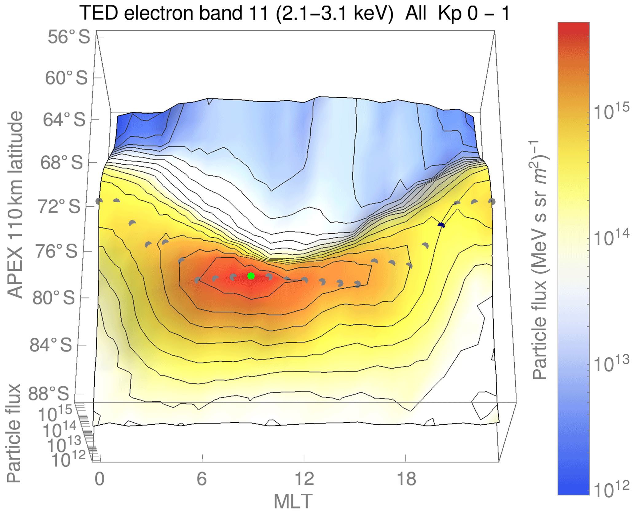
Figure 2Sample for an auroral oval fit. The grey dots represent the position of the auroral oval. The green (9 MLT) and black (20 MLT) dots indicate the maximum and minimum of the auroral oval, respectively.
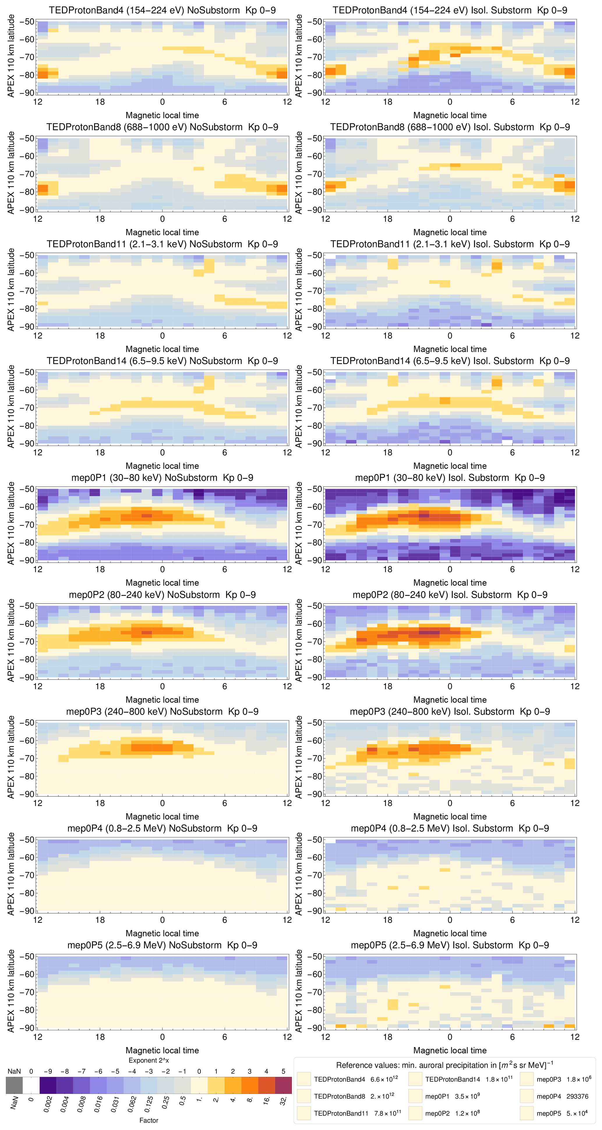
Figure 3 shows the precipitating electron flux at high latitudes in the Southern Hemisphere. The Southern Hemisphere has been chosen to avoid the data gaps between 23 and 1 MLT in the Northern Hemisphere (see Fig. 1, bottom right). Apart from that, the Northern Hemisphere and Southern Hemisphere do not show significant differences in APEX coordinates.
The colour scale is logarithmic with a base of 2, meaning the threshold to the adjacent colour is a factor of 2 apart. The reference value has been set individually for every channel to the lowest occurring value inside the auroral oval. Thus local time differences can be easily identified and quantified. No-substorm periods (left panel) and isolated substorm periods (right panel) for all electron channels are given here.
Figure 4 shows the same as Fig. 3 but for protons.
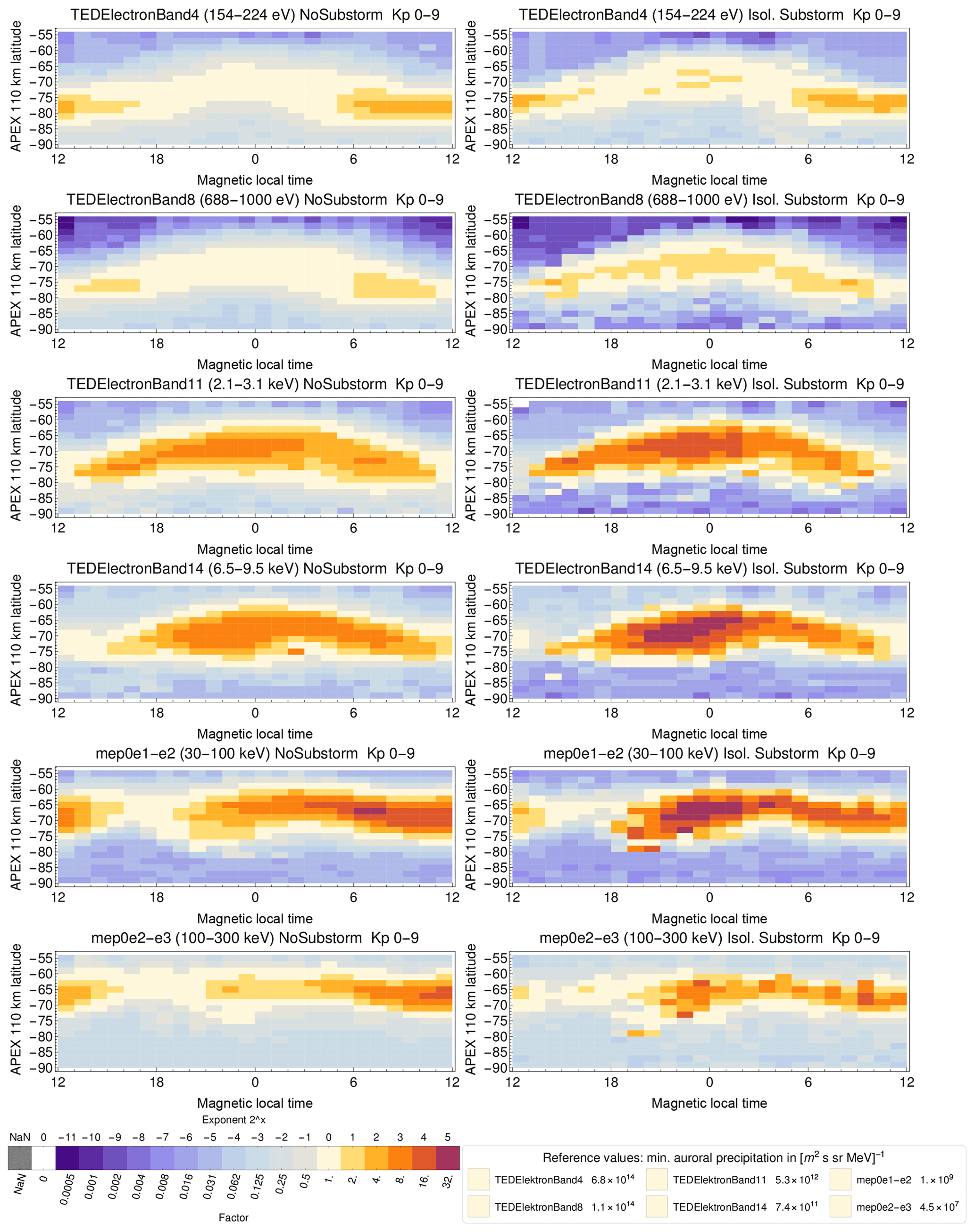
Figure 3Electron flux in various channels at high latitudes in the Southern Hemisphere. The left panel shows periods without substorms and the right panel gives periods with isolated substorms only.
Comparing the two panels of Figs. 3 and 4, we can identify
-
a typical pattern in low energetic channels (see Sect. 4.1),
-
a typical pattern in high energetic channels (see Sect. 4.2),
-
Kp dependence of the auroral MLT asymmetry (see Sect. 4.3),
-
auroral oval asymmetry during substorms (see Sect. 4.4), and
-
a latitudinal displacement of the maximum auroral flux depending on Kp and energy (see Sect. 4.5).
4.1 Typical pattern in low energetic channels
Low energetic proton and electron channels, namely TED electron bands 4 and 8 as well as proton bands 4, 8 and 11, show a very different spatial pattern than the higher channels.
The maximum flux in the auroral oval appears in the day sector. TED electron bands 4 and 8 peak between 6 and 17 MLT. This agrees e.g. very well with the monoenergetic electron number flux for low solar wind driving (Fig. 7 in Newell et al., 2009).
The proton bands are even more concentrated around noon but show an additional slight increase from noon via the morning sector towards midnight. Since this is completely opposite to the higher channels, we will have a look at the source region.
The main precipitation of low energetic electrons (< 1 keV) at daytime (e.g. 76–80∘ S, 6–13 MLT for TED electron band 4) most likely originates from the poleward edge of the cusp, referring to Sandholt et al. (1996, 2000) and Øieroset et al. (1997), who attribute this as a source region during periods with northward Interplanetary Magnetic Field (IMF) (which in our study mostly refers to no-substorm periods as southward IMF triggers substorms).
In contrast, during periods with isolated substorms the particle flux is shifted by 2∘ to the Equator. The source in this case is the equatorward edge of the cusp which has been identified as the corresponding source region in periods of southward IMF by Sandholt and Newell (1992) and Sandholt et al. (1998). A sketch including the source regions may be found in Newell and Meng (1992, Fig. 2), even though the regions are labeled with “Mantle” and “Cusp” here.
In summation our findings confirm that high numbers of low energetic particles enter the magnetosphere preferentially on the front side through cusp and other boundary layers (Newell et al., 2009).
Additionally, low energetic protons (TED proton bands 4–14) show a second oval structure (approx. 50–65∘ S), which is associated with the drift loss cone (see Sect. 3) and thus geographically localized near the SAA. The second oval structure itself is a artifact of the MLT binning (see Fig. 1).
4.2 Typical pattern in high energetic channels
The high electron channels (above >2 keV) show a displacement of the main particle flux with MLT from midnight (TED electron band 11) via the morning sector (mep0e1–e2) to the day sector (mep0e2–e3).
Concerning protons, between TED proton band 14 and the following channels (mep0P1 to mep0P3) the main particle flux shifts from midnight to the evening sector, which is oppositely directed to the electron displacement.
A potential explanation for the displacement in the higher electron channels (and the oppositely directed shift of the protons) is the westward partial ring current in the night side which is closed by field-aligned currents (Birkeland Region 2) into the ionosphere (Lockwood, 2013; Milan et al., 2017). While electrons in the ring current drift eastwards and thus may precipitate predominantly in the morning sector, the protons undergo a westward drift and mainly precipitate in the evening sector. The energy dependence might be due to different drift velocities (Allison et al., 2017). A drift of electron precipitation (>20 keV) towards the dayside has also been reported by Matthews et al. (1988), Newell and Meng (1992) and Østgaard et al. (1999) and is associated with central plasma-sheet electron injections in the midnight region.
The resulting auroral asymmetry also depends on Kp level, as shown in Sect. 4.3.
4.3 Kp dependence of the auroral MLT asymmetry
Even without Kp dependence Figs. 3 and 4 reveal a channel (energy) dependent MLT asymmetry of the particle flux and that the range of this dependence changes with particle energy.
While e.g. the two lowest TED electron channels (bands 4 and 8) show just minor MLT variations, it varies by more than 1 order of magnitude in the higher particle energies.
The proton flux shows distinct MLT dependence, ranging from just minor variations in TED proton bands 11 and 14 (as well as practically no MLT variation in the highest proton MEPED channels) up to about 1 order of magnitude in the lowest and medium particle energies (TED proton bands 4 and 8, MEPED mep0P1 and mep0P3).
During isolated substorms the maximum local time differences are similar or a factor of 2 higher.
However, we noticed that the MLT asymmetry is not constant over different Kp levels. This section will emphasize the impact of Kp levels using Fig. , which is based on the auroral oval determination algorithm from Sect. 3.2 and presents the ratio between maximum and minimum auroral oval fluxes (or in other words, the asymmetry of the oval) depending on Kp level for every channel separately. Actually the channels have been grouped by their Kp dependency. All these findings are based on the whole period, disregarding substorm or not.
The upper panel shows the two lowest electron channels and the lowest proton channel, which all have a declining flux asymmetry with increasing Kp. The 6–6.7 Kp bin is enhanced here, but we should keep in mind that these levels occur rarely and may suffer from bad statistics. A reason for the decline might be that the cusp inflow is not increasing with Kp as the rest of the auroral flux. Thus its relative fraction declines and subsequently decreases the asymmetry.
The middle panel shows all particle channels that have an increasing flux asymmetry with Kp, that is, all remaining electron channels and the proton channels TED band 11 and mep0P1. Given that high geomagnetic disturbance should be linked with enhanced acceleration, scattering and substorm processes increasing asymmetry in the affected regions suggest themselves.
The lowest panel gives the flux asymmetry dependencies of the remaining proton channels that are less distinct. It seems that there is a domain change at about 3.3 Kp since the asymmetry of TED proton band 14 and mep0P2 has a negative correlation below 3.3 and a positive one above. For the channels TED proton band 8 and mep0P3 the relationship is the opposite.
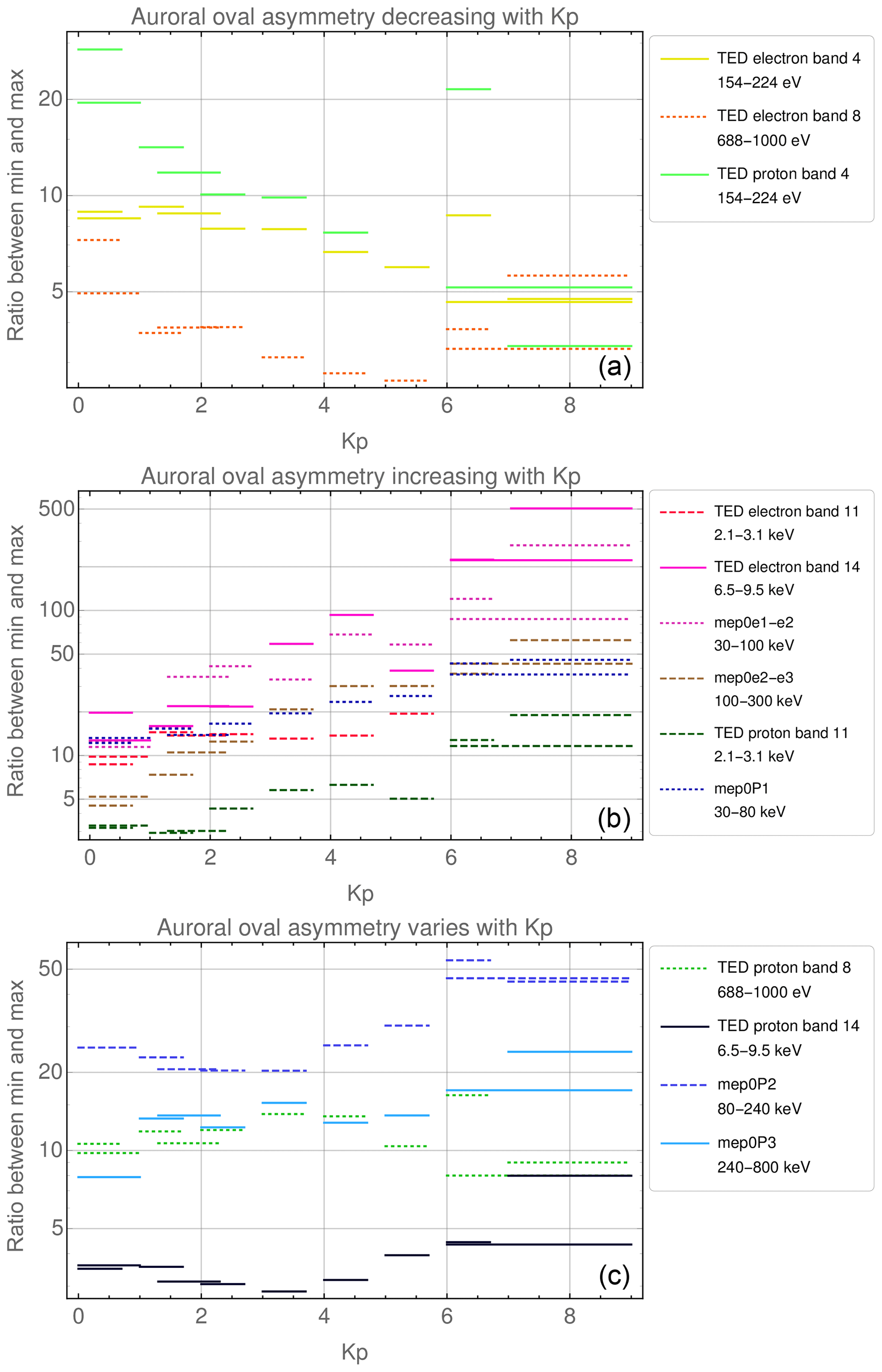
Figure 5Dependence of the auroral oval asymmetry with Kp. (a) Channels whose auroral oval flux shows a negative correlation with Kp, (b) a positive correlation, and (c) no clear correlation.
The two highest energy channels (MEPED mep0P4 and mep0P5) do not show MLT variations as seen in Fig. 4. Particle precipitation is limited to solar proton events. Since these particles enter the ionosphere via open field lines there is no latitudinal focussing but a homogeneous precipitation within the polar cap, which is the reason why the auroral oval fit routine failed and why these channels are not listed in Fig. .
In summation, the maximum MLT asymmetry depends on Kp.
-
For very low energy (proton and electron), it decreases with Kp.
-
For higher electron channels, it increases with Kp.
-
For higher proton channels the Kp dependence is ambiguous, but in general the asymmetry is significantly smaller than in the electron channels.
4.4 Auroral oval asymmetry during substorms
This section discusses the changes during substorm periods based on Figs. 3, 4 and later on Fig. 5.
In general, the particle flux during isolated substorms is similar to no-substorm periods, but is superimposed with substorm-specific night-side (20–2 MLT) particle precipitation, which reflects the substorm electrojet manifestations (Lockwood, 2013; Milan et al., 2017) (see Figs. 3 and 4). In terms of particle acceleration this is the same region that shows Alfvén waves (compare Fig. 4 in Newell et al., 2009) or Alfvénic acceleration (Fig. 14 in Dombeck et al., 2018).
The electron and proton flux intensity at the midnight sector outnumbers the no-substorm values at the same place by factor 2 to 4. For mep0P1 to mep0P3 the evening sector is also slightly increased during substorms. Given the flux increase in the midnight sector, the maximum auroral flux during a substorm can mostly be seen around 0 MLT (see Figs. 3 and 4).
Additionally, noon-sector electron fluxes decrease during a substorm, which is clearly seen in all the upper channels (from TED electron band 11 to mep0e2–e3). The noon-sector flux decreases most probably because dayside particle precipitation occurs often during northward-oriented IMF, which is not usual for substorms (see Fig. 3).
In contrast to the electron fluxes, the day-sector proton fluxes do not significantly depend on substorm activity (see Fig. 4).
Figure 5 presents how the asymmetry depends on substorms. Since an 8-year period does not contain enough values for substorms in rare Kp levels, we neglected the Kp level here and compared isolated substorm to no-substorm periods.
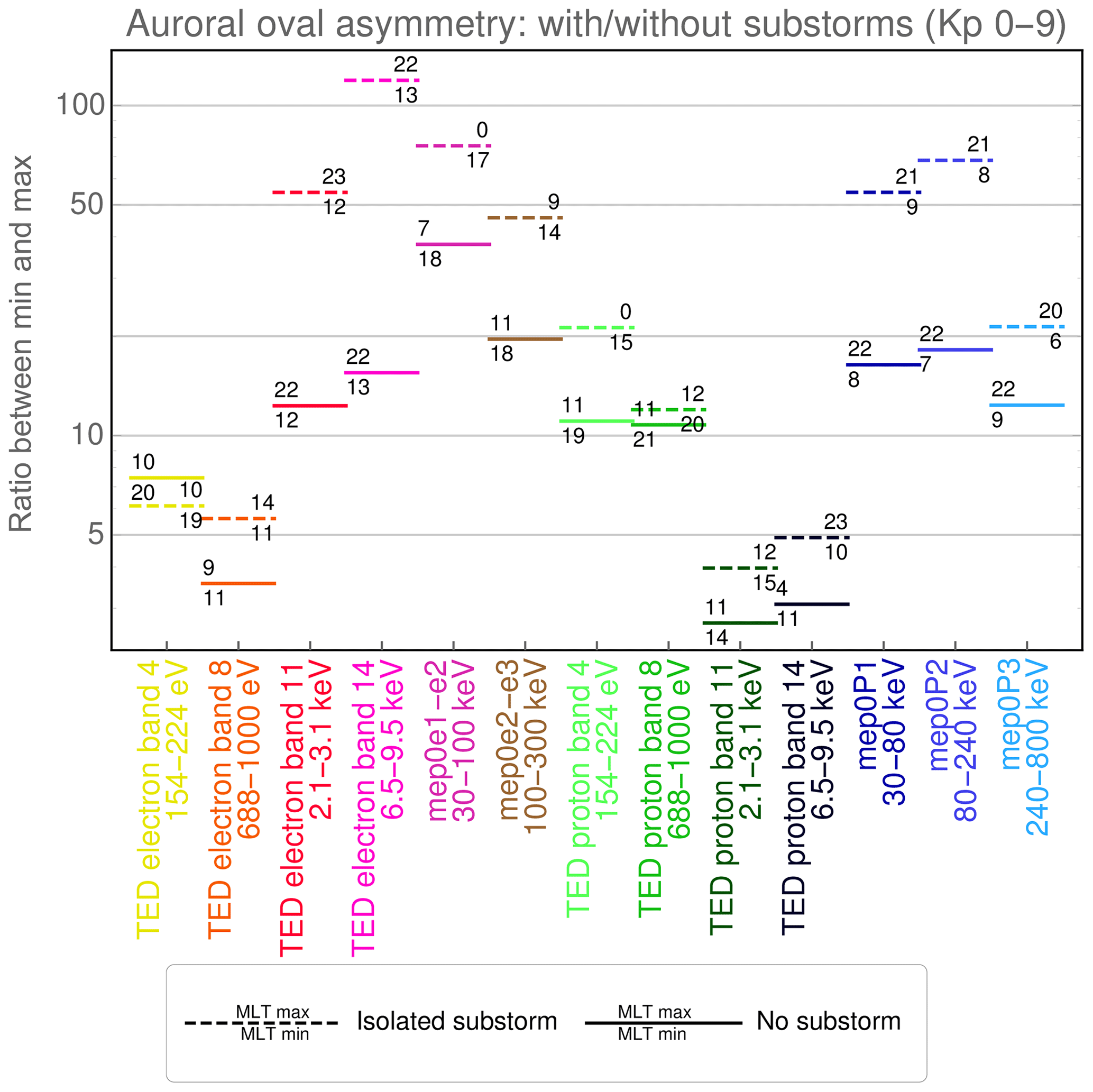
Figure 6The auroral asymmetry is shown as a ratio between maximum and minimum auroral oval fluxes. The number above a specific ratio states the MLT where the maximum is detected, while the number below that ratio indicates the MLT of the minimum.
Except for TED electron band 4 (where there is no significant difference between substorm and no-substorm periods), all other channels have an increased auroral oval asymmetry during isolated substorms. The numbers above and below the marked flux ratio indicate the MLT location of the minimum (below) and maximum (above). We can identify that the maximum flux during a substorm shifts to the midnight sector (if not already there in no-substorm periods), e.g. for mep0e1–e2 or TED protons band 4 and 14.
For TED electron bands 4 and 8 (as well as TED proton bands 8 and 11) the substorm enhancement is also seen in the night sector, but it does not overshoot the dayside flux (see Figs. 3 and 4), while the substorm enhancement in the night sector of mep0e2–e3 is on the same order as the 9–12 MLT flux.
This agrees with Newell et al. (2009), stating that the low energetic particles that enter the magnetosphere at the day side are accelerated by the magnetotail and precipitate at the night side during substorms.
The asymmetry in both the electron and proton spectra (as well as during no-substorm or substorm periods) shows a local minimum in middle TED channels (TED electron band 8 and proton band 11) as well as a local maximum at higher energies (TED electron band 14 or mep0e1–e2 for electron and mep0P1 or mep0P2 for protons). At even higher energies the asymmetry declines again.
4.5 Latitudinal displacement of the maximum auroral flux depending on Kp and energy
Figure 6 presents how the latitude of the maximum auroral oval flux varies with particle energy and Kp. In advance we should note that Fig. 6 may not be over-interpreted since latitudinal displacement of the maximum flux is mainly an effect of a MLT shift (see Fig. 3) that causes the strong latitudinal change between TED electron band 8 and TED electron band 14 for electrons and TED proton band 11 and mep0P1 for protons. Thus the main precipitation zone undergoes a strong latitudinal change, but it does not necessarily describe a latitudinal change in the auroral oval.

Figure 7The modified APEX 110 km latitude of the maximum flux in the auroral oval is shown. Colours indicate specific Kp levels. The left-hand side displays the energy dependence of electrons, the right-hand side the one of the protons.
The figure has been derived by the auroral oval determination method discussed in Sect. 3.2 and displays the latitude of maximum auroral oval flux.
Except for some outliers, most of them belonging to TED proton band 4 during high Kp levels (>6), the graphs show a clear equatorial dislocation with increasing energy. The 110 km APEX latitudinal range at a specific Kp level is about 10∘ for electrons and 12–16∘ for protons. This dislocation however appears to be stepwise: TED electron bands 4 and 8 are almost at the same latitude and TED electron band 14, mep0e1–e2 and mep0e2–e3 share the same latitude. For protons TED proton band 4, 8 and 11 are almost at one latitude and the higher particle energies mep0P1 and mep0P2 are co-located. This implies that these particles originate from the same source population.
However, there is a noticeable latitudinal shift with particle energy even for the particle channels that appear co-located. For 8 out of 11 Kp levels there is an equatorial shift of 2∘ or more between TED electron bands 4 and 8. For protons a latitudinal shift can be recognized between TED proton bands 4 and 11 or between mep0P1 and mep0P3.
Every colour graph represents the spectral location of the maximum flux latitude for a certain Kp range. Thus we can infer that increased geomagnetic disturbance (high Kp values) causes a dislocation of up to about 8∘ towards the Equator.
Concerning the outliers in TED proton band 4, for low Kp values there is a clear flux maximum at noon, which is located at rather high latitudes (compare Fig. 3). At high Kp, the MLT asymmetry declines and then flips. Consequently the maximum flux for high Kp levels is not in the day sector and thus at significantly lower latitudes, but even between the outliers and the maximum flux location in mep0P3 (which is in a similar MLT region) we can recognize a latitudinal shift.
In summation, there is an equatorial shift of the main precipitation zone with increasing Kp and increasing particle energy, while the latter is primarily due to a shift in MLT and only secondarily due to a latitudinal shift of the auroral oval itself.
In this paper we presented the MLT distribution of energetic particle flux/precipitation into the ionosphere in combination with different substorm activity.
We could identify low energetic particles to predominantly precipitate around local noon, supporting the idea that they enter the magnetosphere through the cusp. During substorms the maximum particle flux is shifted by 2∘ to the Equator.
Higher particle energies show a different behaviour. Electrons (>2 keV) mainly precipitate at midnight, but with increasing particle energy the maximum flux shifts via the morning sector to the day sector. Maximum proton flux, on the other hand, shifts from the midnight sector to the evening sector with increasing energy. A drift of electron precipitation (>20 keV) towards the dayside is associated with central plasma-sheet electron injections in the midnight region.
There is an energy-dependent auroral asymmetry. While the low energetic electrons have just a minor asymmetry, it enhances to more than 1 order of magnitude for the higher electron channels. For low energetic protons the cusp precipitation causes an asymmetry of about an order of magnitude. Above that energy the asymmetry first declines (to factor 2 in TED proton bands 11 and 14) and then enlarges again with MEPED channels 1 to 3 (more than an order of magnitude). For the highest proton channels the asymmetry disappears as these particles are not linked with auroral precipitation. During substorms the maximum flux is similar or a factor 2 higher.
The auroral asymmetry is Kp-dependent. For low energetic particles the asymmetry declines with Kp, probably due to a lack of cusp precipitation during high Kp values, while it increases especially (stronger) for higher electron channels, probably due to increased acceleration and scattering processes. For medium and high energetic protons the development of the asymmetry with Kp is not that distinct; there might be multiple processes involved.
During substorms the no-substorm flux seems to be generally superimposed by substorm-specific night-side particle flux. However, the noon-sector fluxes depend on particle species. For protons they seem to be independent of substorm activity, while for electrons they decrease during a substorm.
Also, we noticed a Kp- and energy-dependent equatorial shift of the main flux latitude.
Upon request, the data used for the publication of this study are available from the authors: Olesya Yakovchuk (oyakovchuk@uos.de) or Jan Maik Wissing (jawissin@uos.de).
The authors worked on all parts of the paper jointly.
The authors declare that they have no conflict of interest.
This article is part of the special issue “Vertical coupling in the atmosphere–ionosphere system”. It is a result of the 7th Vertical Coupling workshop, Potsdam, Germany, 2–6 July 2018.
The authors acknowledge the NOAA National Centers for Environmental Information (https://ngdc.noaa.gov/stp/satellite/poes/dataaccess.html, last access: 26 November 2019) for the POES and METOP particle data used in this study and give many thanks to the SuperMAG team (http://supermag.jhuapl.edu/, last access: 26 November 2019) and their collaborators (http://supermag.jhuapl.edu/info/?page=acknowledgement, last access: 26 November 2019).
The work is supported by DFG project WI4417/2-1.
This research has been supported by the German Science Foundation (DFG; grant no. WI4417/2-1).
This open-access publication was funded
by Osnabrück University.
This paper was edited by Elias Roussos and reviewed by two anonymous referees.
Akasofu, S.-I.: The development of the auroral substorm, Planet. Space Sci., 12, 273–282, https://doi.org/10.1016/0032-0633(64)90151-5, 1964. a
Akasofu, S.-I.: Auroral substorms as an electrical discharge phenomenon, Progress in Earth and Planetary Science, 2, 20, https://doi.org/10.1186/s40645-015-0050-9, 2015. a
Akasofu, S. I., Chapman, S., and Meng, C. I.: The polar electrojet, J. Atmos. Terr. Phys., 27, 1275–1300, https://doi.org/10.1016/0021-9169(65)90087-5, 1965. a
Allison, H. J., Horne, R. B., Glauert, S. A., and Del Zanna, G.: The magnetic local time distribution of energetic electrons in the radiation belt region, J. Geophys. Res.-Space, 122, 8108–8123, https://doi.org/10.1002/2017JA024084, 2017. a, b
Asikainen, T., Mursula, K., and Maliniemi, V.: Correction of detector noise and recalibration of NOAA/MEPED energetic proton fluxes, J. Geophys. Res., 117, A09204, https://doi.org/10.1029/2012JA017593, 2012. a
Bartels, J., Heck, N. H., and Johnston, H. F.: The three-hour-range index measuring geomagnetic activity, Terrestrial Magnetism and Atmospheric Electricity, 44, 411, https://doi.org/10.1029/TE044i004p00411, 1939. a
Berkey, F. T., Driatskiy, V. M., Henriksen, K., Hultqvist, B., Jelly, D. H., Shchuka, T. I., Theander, A., and Ylindemi, J.: A synoptic investigation of particle precipitation dynamics for 60 substorms in IQSY (1964–1965) and IASY (1969), Planet. Space Sci., 22, 255–307, https://doi.org/10.1016/0032-0633(74)90028-2, 1974. a
Birn, J., Thomsen, M. F., Borovsky, J. E., Reeves, G. D., McComas, D. J., and Belian, R. D.: Characteristic plasma properties during dispersionless substorm injections at geosynchronous orbit, J. Geophys. Res., 102, 2309–2324, https://doi.org/10.1029/96JA02870, 1997. a
Bornebusch, J., Wissing, J., and Kallenrode, M.-B.: Solar particle precipitation into the polar atmosphere and their dependence on hemisphere and local time, Adv. Space Res., 45, 632–637, https://doi.org/10.1016/j.asr.2009.11.008, 2010. a
Callis, L. B., Baker, D. N., Natarajan, M., Bernard, J. B., Mewaldt, R. A., Selesnick, R. S., and Cummings, J. R.: A 2-D model simulation of downward transport of NOy into the stratosphere: Effects on the 1994 austral spring O3 and NOy, Geophys. Res. Lett., 23, 1905–1908, https://doi.org/10.1029/96GL01788, 1996a. a
Callis, L. B., Boughner, R. E., Baker, D. N., Mewaldt, R. A., Bernard Blake, J., Selesnick, R. S., Cummings, J. R., Natarajan, M., Mason, G. M., and Mazur, J. E.: Precipitating electrons: Evidence for effects on mesospheric odd nitrogen, Geophys. Res. Lett., 23, 1901–1904, https://doi.org/10.1029/96GL01787, 1996b. a
Davis, T. N. and Sugiura, M.: Auroral electrojet activity index AE and its universal time variations, J. Geophys. Res., 71, 785–801, https://doi.org/10.1029/JZ071i003p00785, 1966. a
Dombeck, J., Cattell, C., Prasad, N., Meeker, E., Hanson, E., and McFadden, J.: Identification of Auroral Electron Precipitation Mechanism Combinations and Their Relationships to Net Downgoing Energy and Number Flux, J. Geophys. Res.-Space, 123, 10, https://doi.org/10.1029/2018JA025749, 2018. a, b
Evans, D. S. and Greer, M. S.: Polar Orbiting Environmental Satellite Space Environment Monitor – 2, Instrument Descriptions and Archive Data Documentation, National Oceanic and Atmospheric Administration, NOAA Space Environ. Lab, Boulder, Colorado, USA, version 1.4b, including TED calibrations, 2004. a
Evans, D. S. and Greer, M. S.: Polar Orbiting Environmental Satellite Space Environment Monitor – 2, Instrument Descriptions and Archive Data Documentation, National Oceanic and Atmospheric Administration, NOAA Space Environ. Lab, Boulder, Colorado, USA, version 2.0, 2006. a, b, c, d, e
Frank, L. A., Craven, J. D., Ackerson, K. L., English, M. R., Eather, R. H., and Carovillano, R. L.: Global auroral imaging instrumentation for the Dynamics Explorer Mission, Space Science Instrumentation, 5, 369–393, 1981. a
Fujii, R., Hoffman, R. A., Anderson, P. C., Craven, J. D., Sugiura, M., Frank, L. A., and Maynard, N. C.: Electrodynamic parameters in the nighttime sector during auroral substorms, J. Geophys. Res., 99, 6093–6112, https://doi.org/10.1029/93JA02210, 1994. a
Gjerloev, J. W., Hoffman, R. A., Friel, M. M., Frank, L. A., and Sigwarth, J. B.: Substorm behavior of the auroral electrojet indices, Ann. Geophys., 22, 2135–2149, https://doi.org/10.5194/angeo-22-2135-2004, 2004. a
Hardy, D. A., Gussenhoven, M. S., and Holeman, E.: A statistical model of auroral electron precipitation, J. Geophys. Res., 90, 4229–4248, https://doi.org/10.1029/JA090iA05p04229, 1985. a
Heath, D. F., Krueger, A. J., and Crutzen, P. J.: Solar proton event – Influence on stratospheric ozone, Science, 197, 886–889, https://doi.org/10.1126/science.197.4306.886, 1977. a
Lockwood, M.: Reconstruction and Prediction of Variations in the Open Solar Magnetic Flux and Interplanetary Conditions, Living Rev. Sol. Phys., 10, 4, https://doi.org/10.12942/lrsp-2013-4, 2013. a, b
Logachev, Y. I., Bazilevskaya, G. A., Vashenyuk, E. V., Daibog, E. I., Ishkov, V. N., Lazutin, L. L., Miroshnichenko, L. I., Nazarova, M. N., Petrenko, I. E., Stupishin, A. G., Surova, G. M., and Yakovchuk, O. S.: Catalog of solar proton events in the 23rd cycle of solar activity (1996–2008), The Geophysical Center of the Russian Academy of Sciences, 743, https://doi.org/10.2205/ESDB-SAD-P-001-RU, 2016. a
Matthews, D. L., Rosenberg, T. J., Benbrook, J. R., and Bering III, E. A.: Dayside energetic electron precipitation over the South Pole (lambda = 75 deg), J. Geophys. Res., 93, 12941–12945, https://doi.org/10.1029/JA093iA11p12941, 1988. a
McPherron, R. L.: Growth phase of magnetospheric substorms, J. Geophys. Res., 75, 5592, https://doi.org/10.1029/JA075i028p05592, 1970. a
Mende, S. B., Frey, H. U., Morsony, B. J., and Immel, T. J.: Statistical behavior of proton and electron auroras during substorms, J. Geophys. Res.-Space, 108, 1339, https://doi.org/10.1029/2002JA009751, 2003. a
Meredith, N. P., Horne, R. B., Lam, M. M., Denton, M. H., Borovsky, J. E., and Green, J. C.: Energetic electron precipitation during high-speed solar wind stream driven storms, J. Geophys. Res.-Space, 116, A05223, https://doi.org/10.1029/2010JA016293, 2011. a
Milan, S. E., Clausen, L. B. N., Coxon, J. C., Carter, J. A., Walach, M.-T., Laundal, K., Østgaard, N., Tenfjord, P., Reistad, J., Snekvik, K., Korth, H., and Anderson, B. J.: Overview of Solar Wind-Magnetosphere-Ionosphere-Atmosphere Coupling and the Generation of Magnetospheric Currents, Space Sci. Rev., 206, 547–573, https://doi.org/10.1007/s11214-017-0333-0, 2017. a, b
Newell, P. T. and Gjerloev, J. W.: Evaluation of SuperMAG auroral electrojet indices as indicators of substorms and auroral power, J. Geophys. Res.-Space, 116, A12211, https://doi.org/10.1029/2011JA016779, 2011a. a, b, c
Newell, P. T. and Gjerloev, J. W.: Substorm and magnetosphere characteristic scales inferred from the SuperMAG auroral electrojet indices, J. Geophys. Res.-Space, 116, A12232, https://doi.org/10.1029/2011JA016936, 2011b. a
Newell, P. T. and Meng, C.-I.: Mapping the dayside ionosphere to the magnetosphere according to particle precipitation characteristics, J. Geophys. Res., 19, 609–612, https://doi.org/10.1029/92GL00404, 1992. a, b
Newell, P. T., Sotirelis, T., and Wing, S.: Diffuse, monoenergetic, and broadband aurora: The global precipitation budget, J. Geophys. Res.-Space, 114, A09207, https://doi.org/10.1029/2009JA014326, 2009. a, b, c, d, e, f
Newell, P. T., Lee, A. R., Liou, K., Ohtani, S.-I., Sotirelis, T., and Wing, S.: Substorm cycle dependence of various types of aurora, J. Geophys. Res.-Space, 115, A09226, https://doi.org/10.1029/2010JA015331, 2010. a
Øieroset, M., Sandholt, P. E., Denig, W. F., and Cowley, S. W. H.: Northward interplanetary magnetic field cusp aurora and high-latitude magnetopause reconnection, J. Geophys. Res., 102, 11349–11362, https://doi.org/10.1029/97JA00559, 1997. a
Østgaard, N., Stadsnes, J., Bjordal, J., Vondrak, R. R., Cummer, S. A., Chenette, D. L., Parks, G. K., Brittnacher, M. J., and McKenzie, D. L.: Global-scale electron precipitation features seen in UV and X rays during substorms, J. Geophys. Res., 104, 10191–10204, https://doi.org/10.1029/1999JA900004, 1999. a
Reeves, G. D., Henderson, M. G., Skoug, R. M., Thomsen, M. F., Borovsky, J. E., Funsten, H. O., Son Brandt, P. C., Mitchell, D. J., Jahn, J.-M., Pollock, C. J., McComas, D. J., and Mende, S. B.: IMAGE, POLAR, and Geosynchronous Observations of Substorm and Ring Current Ion Injection, in: Disturbances in Geospace: The Storm-substorm Relationship, edited by: Surjalal Sharma, A., Kamide, Y., and Lakhina, G. S., Vol. 142 of Washington DC American Geophysical Union Geophysical Monograph Series, p. 91, https://doi.org/10.1029/142GM09, 2003. a
Richmond, A. D.: Ionospheric Electrodynamics Using Magnetic Apex Coordinates, J. Geomagn. Geoelectr., 47, 191–212, https://doi.org/10.5636/jgg.47.191, 1995. a, b, c
Rodger, C. J., Clilverd, M. A., Green, J. C., and Lam, M. M.: Use of POES SEM-2 observations to examine radiation belt dynamics and energetic electron precipitation into the atmosphere, J. Geophys. Res.-Space, 115, A04202, https://doi.org/10.1029/2008JA014023, 2010. a, b, c
Sandholt, P. E. and Newell, P. T.: Ground and satellite observations of an auroral event at the cusp/cleft equatorward boundary, J. Geophys. Res., 97, 8685–8691, https://doi.org/10.1029/91JA02995, 1992. a
Sandholt, P. E., Farrugia, C. J., Øieroset, M., Stauning, P., and Cowley, S. W. H.: Auroral signature of lobe reconnection, Geophys. Res. Lett., 23, 1725–1728, https://doi.org/10.1029/96GL01846, 1996. a
Sandholt, P. E., Farrugia, C. J., Moen, J., and Cowley, S. W. H.: Dayside auroral configurations: Responses to southward and northward rotations of the interplanetary magnetic field, J. Geophys. Res., 103, 20279–20296, https://doi.org/10.1029/98JA01541, 1998. a
Sandholt, P. E., Farrugia, C. J., Cowley, S. W. H., Lester, M., Denig, W. F., Cerisier, J.-C., Milan, S. E., Moen, J., Trondsen, E., and Lybekk, B.: Dynamic cusp aurora and associated pulsed reverse convection during northward interplanetary magnetic field, J. Geophys. Res., 105, 12869–12894, https://doi.org/10.1029/2000JA900025, 2000. a
Thorne, R. M.: Energetic radiation belt electron precipitation – A natural depletion mechanism for stratospheric ozone, Science, 195, 287–289, https://doi.org/10.1126/science.195.4275.287, 1977. a
Wissing, J. M., Bornebusch, J., and Kallenrode, M.-B.: Variation of energetic particle precipitation with local magnetic time, Adv. Space Res., 41, 1274–1278, https://doi.org/10.1016/j.asr.2007.05.063, 2008. a
Yando, K., Millan, R. M., Green, J. C., and Evans, D. S.: A Monte Carlo simulation of the NOAA POES Medium Energy Proton and Electron Detector instrument, J. Geophys. Res.-Space, 116, A10231, https://doi.org/10.1029/2011JA016671, 2011. a