the Creative Commons Attribution 4.0 License.
the Creative Commons Attribution 4.0 License.
 | 26 Jun 2018
Comparison of H component geomagnetic field time series obtained at different sites over South America
Maurício J. A. Bolzan
Clezio M. Denardini
Alexandre Tardelli
The geomagnetic field in the Brazilian sector is influenced by the South American Magnetic Anomaly (SAMA) that causes a decrease in the magnitude of the local geomagnetic field when compared to other regions in the world. Thus, the magnetometer network and data set of space weather over Brazil led by Embrace are important tools for promoting the understanding of geomagnetic fields over Brazil. In this sense, in this work we used the H component of geomagnetic fields obtained at different sites in South America in order to compare results from the phase coherence obtained from wavelet transform (WT). Results from comparison between Cachoeira Paulista (CXP) and Eusébio (EUS), and Cachoeira Paulista and São Luis (SLZ), indicated that there exist some phenomena that occur simultaneously in both locations, putting them in the same phase coherence. However, there are other phenomena putting both locations in a strong phase difference as observed between CXP and Rio Grande, Argentina (RGA). This study was done for a specific moderate geomagnetic storm that occurred in March 2003. The results are explained in terms of nonlinear interaction between physical phenomena acting in distinct geographic locations and at different times and scales.
Keywords. Geomagnetism and paleomagnetism (time variations – diurnal to secular)


The use of the magnetosphere time series is important for understanding the important geophysical phenomenon called the South American Magnetic Anomaly (SAMA) and the impact of the perturbations of the coronal mass ejections (CMEs) (Klausner et al., 2016, and references therein). Predictions from models (Bilitza, 2001) provide good agreement with the experimental results. The increase in the sensitivity of these models indicates the necessity of more detailed studies of the intermittent phenomena present in the geomagnetic system (Bolzan et al., 2005, 2009, 2012).
Some works have been carried out in the geomagnetic system in order to obtain characteristics for forecasting. Papa et al. (2006), studying the geomagnetic time series obtained in Brazil, showed that the power-law regime changes are good indications of the incoming disturbance in the geomagnetic system. Also, Papa and Sosman (2008), using data from magnetometers recorded at Vassouras (VSS) and the Dst index time series, have shown the possibility of envisaging a probabilistic forecasting method. These results have shown the possibility of predicting the incoming geomagnetic disturbance. However, several physical factors depend upon a useful predictability, such as the frozen magnetic field inside the CMEs. Over South America other factors become important, such as the presence of the SAMA where the geomagnetic field is the weakest in the world. Thus, the study of the energy transfer process from the CME to inside the coupled magnetosphere–ionosphere system over Brazil is a rich area of research. Besides, it allows us to understand and prevent technological issues like interruption in satellite communications, power-line transmission blackout, and positioning degradations for those GNSS satellite-based positioning systems. One tool for studying such coupling is the wavelet-coherence phase difference.
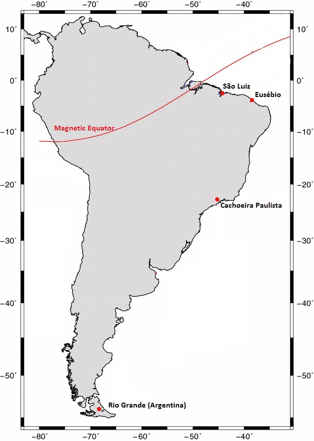
Figure 1Locations of the magnetometer stations in South America (source: adapted from Padilha et al., 2017).
Recently, a new magnetometer network in Brazil and Latin America was created, led by Embrace from the National Institute for Space Research (INPE) along with the Universidade do Vale do Paraíba (UNIVAP), with several participants from Latin America. The network covers a range of approximately 50∘ × 40∘ (latitude and longitude) in the South American sector (Denardini et al., 2018a) and is part of an international effort to provide results that are comparable to the absolute measurements made at magnetic observatories, which are suitable for space weather studies (Denardini et al., 2018b). Denardini et al. (2016a, b) also published a review of this subject and the regional efforts that have been made to build a magnetometer network as well as provide some information on Fabry–Pérot interferometers, ionosonde, and all-sky imagers, installed over Latin America, and their importance in improving the space weather forecast in this region. The data collected by most of the instruments of the Embrace network are available online at the website http://www.inpe.br/spaceweather, last access: 30 March 2015.
We have used the H component of geomagnetic field time series of the following observatories, at one measurement per minute during March 2003, obtained at Cachoeira Paulista (CXP, 22.67∘ S, 44.99∘ W, dip: −22.0), São Luis (SLZ, 2.3∘ S, 44.2∘ W, dip: −7.21), Eusébio (EUS, 3.89∘ S, 38.2∘ W, dip: −16.51), and Rio Grande, Argentina (RGA, 53.78∘ S, 67.7∘ W, dip: −50.03). Figure 1 shows the map with the magnetometer stations in South America (for more details about the magnetic stations, see Denardini et al., 2015, 2016a, b, c). This set of data was chosen based on the availability of the data and due to the presence of a moderated geomagnetic storm that occurred on 15 March 2003, as can be identified in Fig. 2. Despite this geomagnetic storm being moderated (Dst > −100 nT), the measurement made in the eastern American sector seems to have been strong due to the presence of a sharp and strong decrease at the H component, as we will investigate in this work.
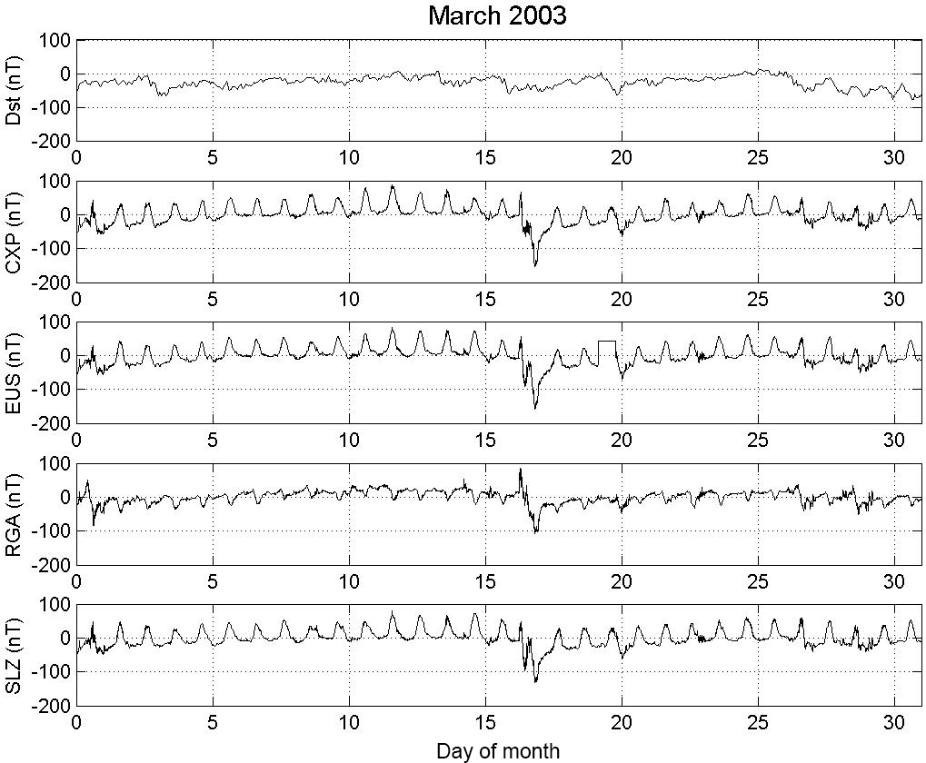
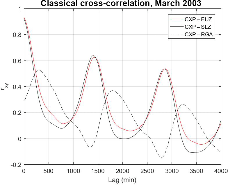
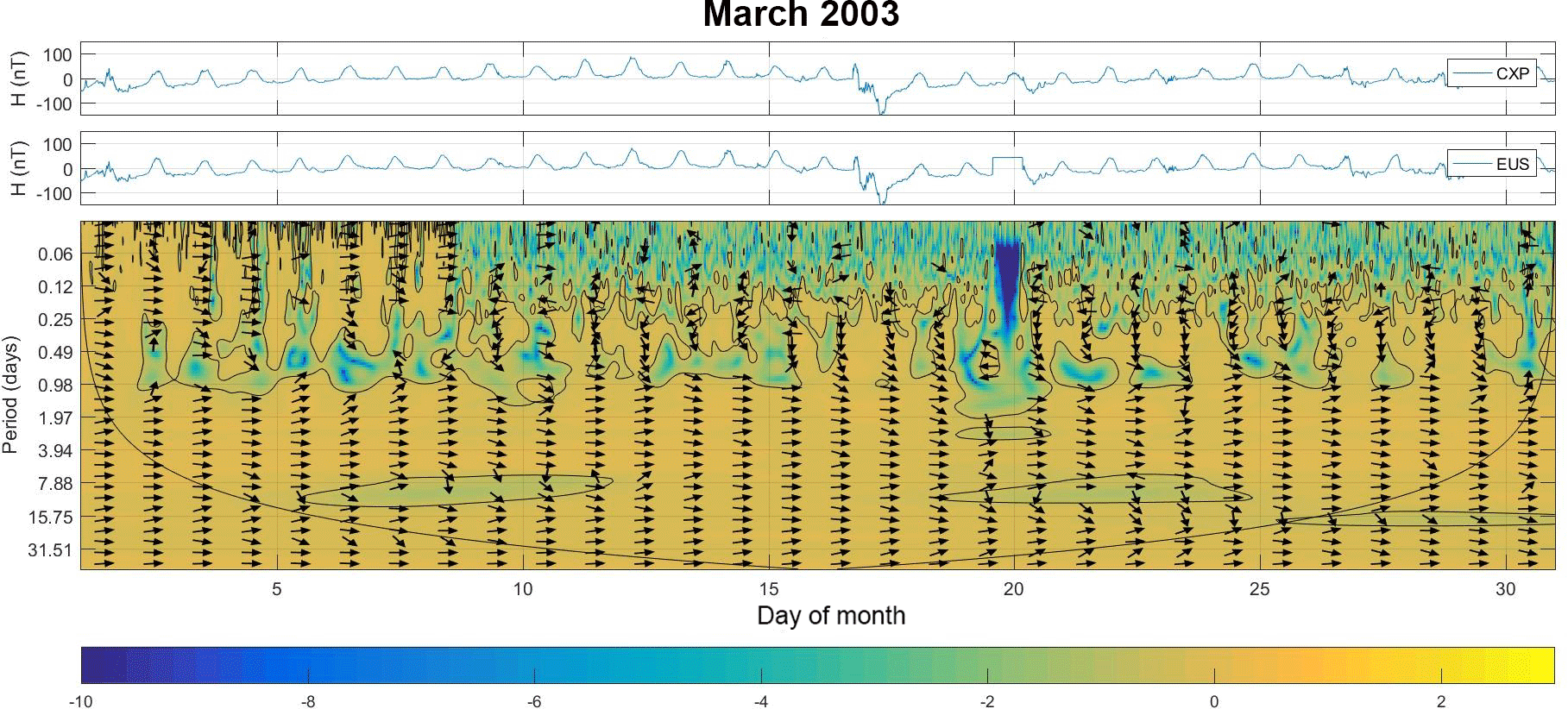
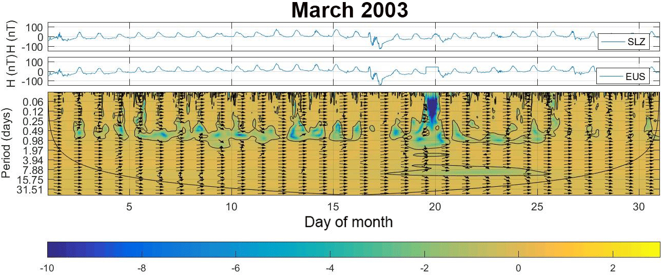
Figure 4(a) Monthly time series of the H component from the geomagnetic field of the CXP and EUS, Brazil; (b) phase coherence applied in the same time series. Arrows indicate the phase difference between the time series of the wavelet spectra where right arrows indicate series are in phase, left arrows indicate series are completely out of phase (180∘), and an arrow pointing vertically means the second series lags the first by 90∘.
3.1 Classical cross-correlation analysis
The classical cross-correlation was used in order to obtain the time lags where the time series presented high and/or low correlations. This mathematical tool is useful for giving us the first insight into both time series where the 0 value indicates no correlation between time series, the 1 value indicates a perfect correlation, and the −1 value indicates a total anti-correlation. The mathematical formulation is given by
where x(n) and y(n) are the two time series, and l is the time lag used to perform the cross-correlation.
As mentioned before, this classical formalism of the cross-correlation is an important tool for giving us information about the time-lag correlation between two time series. However, this tool is not able to give information about the periodicities where two time series are correlated or not; i.e., it is not possible to infer temporal scales where the correlations are strong or weak. Thus, we used the wavelet cross-correlation, which is a good mathematical tool able to give the information of the correlations by scale. In the next section we present a brief introduction to this subject.
3.2 Cross-wavelet analysis
The time series obtained from any natural system are non-stationary; i.e., the statistical moments from superior orders are not constant. Thus, the use of traditional mathematical tools such as fast Fourier transform (FFT) are not appropriate for non-stationary time series. This problem was resolved in the 1980s through the introduction of appropriate mathematical functions able to give the energy temporal variability for each frequency present in the time series. Thus, we present a brief introduction to this robust mathematical tool used in this work.
We used the Morlet wavelet transform to obtain the temporal variability of the main periodicities and, also, the phase coherence. The Morlet function is given by
and the wavelet transform is given by
where a is the dilation parameter or factor scale, b is the location parameter, Ψ∗ is the complex conjugate of the wavelet function, and f(t) is the time series.
In order to obtain the phase coherence from wavelet transform, we used the coherence phase suggested by Liu (1994), mentioned by Torrence and Compo (1998):
where a is the scaling factor and WXY the cross-wavelet transform applied in two time series given by (Torrence and Compo, 1998; Bolzan and Vieira, 2006)
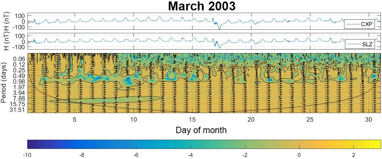
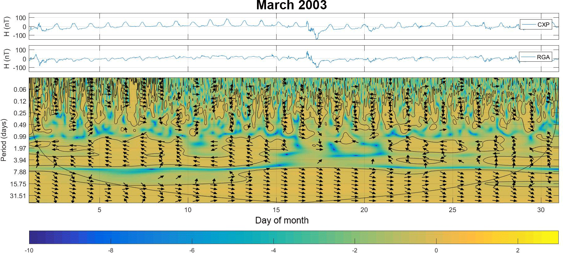
where ∗ means the complex conjugate of the wavelet transform. The phase coherence applied to time series between CXP and EUS, CXP and SLZ, EUS and SLZ, and CXP and RGA is shown in Figs. 3, 4, 5, and 6, respectively.

The classical cross-correlation is used as a first statistical analysis in order to observe the main temporal scales where two time series are correlated, anti-correlated, or non-correlated. Figure 3 shows the results between the following time series: CXP-EUS, CXP-SLZ, CXP-RGA, where it is possible to see a good correlation between CXP-EUS and CXP-SLZ at initial time lags with values near to 1 and other maxima every 1440 min as expected due to the diurnal variation. Furthermore, we observe a low anti-correlation between the CXP-RGA every 1440 min; i.e., both time series are out of phase of 180∘. Despite this anti-correlation being expected since models have predicted that the focus of the daytime Southern Hemisphere ionospheric current sheet would be located more northerly than RGA but more southerly than the other stations, this is the first time that this has been measured in South America and proven based on wavelet analysis. In physical terms the wavelet anti-correlation result is indicative that the ionospheric currents are eastward at low latitudes and westward at high latitudes where RGA is situated. Despite these results, we were not able to understand how this phase difference occurs in terms of the different periods (timescales or vertical scale in the maps) presented in the wavelet map analysis. Thus, in order to quantify these results associated with scales and phase coherence, the cross-wavelet transform was used.
Results from the wavelet-coherence phase difference for CXP–EUS and CXP–SLZ have shown that these time series are in phase for any periodicity scales, according to arrows pointing right. This fact corroborates the statement that these three stations are set under the same eastward ionospheric current influence, leading to the good correlation and the same phase coherence as observed in Figs. 3, 4, 5, and 6. We observe low cross-correlation on a 1-day scale even if both time series present the same periodicity. Another interesting point is due to the low cross-correlation in 8-day periodicity between time series from EUS and CXP 5 days (approximately) before the incoming geomagnetic disturbance. The same behavior was also observed between time series from SLZ and CXP, also 5 days before the incoming geomagnetic disturbance and for 8-day periodicity.
In order to analyze the behavior of the two stations close to the equatorial electrojet (EEJ) such as EUS and SLZ, we performed the coherence phase difference for both these stations. Figure 4 shows the results where it is interesting to note that both time series are in phase during all the time and all periodicities, except for semi and diurnal variations. We observe a low cross-correlation between scales 8 to 16 days after the geomagnetic storm and continue for 5 days after this event.
Afterwards, we performed a comparison between CXP and RGA, which are two stations located really far from each other. Figure 7 shows distinct behavior when compared to the other cases already analyzed. We note that both time series present a difference phase of 180∘ for scales lower than 8 days, and they are in phase for larger scales. The reason we obtain a difference phase of 180∘ can be explained through the clockwise ionospheric currents that took place in the Southern Hemisphere on smaller scales. These ionospheric currents were extensively studied by Alberti et al. (2016). This subject about the ionospheric currents is very interesting due to its importance in ionosphere–magnetosphere coupling (Stening et al., 2007), but it is less explored over the SAMA region. In order to analyze this aspect of the difference phase of 180∘ for other cases, we applied the same procedure for the whole month of January 2016. We chose this month due to the presence of a geomagnetic substorm that occurred in the second part of this month. Figure 8 shows the wavelet coherence phase difference for SLZ–RGA where we can observe a difference phase of 180∘ for scales lower than 8 days and in phase for larger scales also. Thus, we can conjecture that these results between SLZ and RGA are due to the clockwise ionospheric currents that took place in the Southern Hemisphere on smaller scales. This is an important conclusion from this work, i.e., to characterize the clockwise ionospheric currents in the Southern Hemisphere.
It is important to note that the periods found in this work are according to the Nyquist sampling theorem which states that the sampling frequency should be at least twice the highest frequency contained in the signal. Thus, the sample size of our time series (31 days) does not introduce artifacts due to the processing wavelet software in scales ∼ 8 days because this scale is almost 4 times lower when compared with a 31-day scale.
In summary, the latitudinal extension magnetometer network over South America led by Embrace allows us to study several physical phenomena such as the ionospheric current distribution over this region where the SAMA is located. The classical cross-correlation and cross-wavelet performed between some chosen stations have shown the following results.
-
Magnetometers located inside the low-latitude region are very well correlated and are in the same coherence phase.
-
Magnetometers located in regions where the ionospheric currents are in opposite directions such as Cachoeira Paulista and Rio Grande have shown a good correlation but 180∘ difference phase for timescales lower than 8 days (1 week approximately).
-
It was very interesting to observe that the presence of strong oscillations, such as a geomagnetic disturbance, put all magnetometer stations in the same phase due to this physical phenomenon.
-
Another important highlight of this work is the possibility of characterizing the clockwise ionospheric currents in the Southern Hemisphere. Furthermore, it will be possible to study the effect of the geomagnetic substorm effects on these currents in future works. This fact was observed in two distinct geomagnetic storms.
In future works we will apply the discrete wavelet analysis, using the Haar function, in order to calculate what the scales are between stations that show stronger correlation. This will be a similar analysis to this work.
All data used to produce the results of this paper were obtained from EMBRACE/INPE through the web site http://www2.inpe.br/climaespacial/portal/variacao-de-h/, last access: 21 March 2015.
MJAB designed and analyzed the work, and wrote the paper. CMD also analyzed the work and wrote the paper. AT helped with analysis also.
The authors declare that they have no conflict of interest.
This article is part of the special issue “Space weather connections to near-Earth space and the atmosphere”. It is a result of the 6∘ Simpósio Brasileiro de Geofísica Espacial e Aeronomia (SBGEA), Jataí, Brazil, 26–30 September 2016.
Maurício J. A. Bolzan was supported by CNPq agency contract number
302330/2015-1 and FAPEG agency contract number 2012.1026.7000905.
Clezio M. Denardini thanks CNPq/MCTI (grant 03121/2014-9) and FAPESP
(grant 2012/08445-9). Alexandre Tardelli was supported by FAPESP
(grant 2015/24791-2). The authors thank Embrace/INPE and ISGS for providing
the geomagnetic data and the SSC information, respectively. The authors thank
editor Alisson Dal Lago and anonymous referees for help in evaluating this
paper.
The topical editor,
Alisson Dal Lago, thanks two anonymous referees for help in evaluating this
paper.
Alberti, T., Piersanti, M., Vecchio, A., De Michelis, P., Lepreti, F., Carbone, V., and Primavera, L.: Identification of the different magnetic field contributions during a geomagnetic storm in magnetospheric and ground observations, Ann. Geophys., 34, 1069–1084, https://doi.org/10.5194/angeo-34-1069-2016, 2016.
Bilitza, D.: International Reference Ionosphere 2000, Radio Sci., 36, 261–275, https://doi.org/10.1029/2000RS002432, 2001.
Bolzan, M. J. A. and Rosa, R. R.: Multifractal analysis of interplanetary magnetic field obtained during CME events, Ann. Geophys., 30, 1107–1112, https://doi.org/10.5194/angeo-30-1107-2012, 2012.
Bolzan, M. J. A. and Vieira, P. C.: Wavelet analysis of the wind velocity and temperature variability in the Amazon forest, Braz. J. Phys., 36, 1217–1222, https://doi.org/10.1590/S0103-97332006000700018, 2006.
Bolzan, M. J. A., Sahai, Y., Fagundes, P. R., Rosa, R. R., Ramos, F. M., and Abalde, J. R.: Intermittency analysis of geomagnetic storm time-series observed in Brazil, J. Atmos. Sol.-Terr. Phy., 67, 1365–1372, https://doi.org/10.1016/j.jastp.2005.06.008, 2005.
Bolzan, M. J. A., Rosa, R. R., and Sahai, Y.: Multifractal analysis of low-latitude geomagnetic fluctuations, Ann. Geophys., 27, 569–576, https://doi.org/10.5194/angeo-27-569-2009, 2009.
Denardini, C. M., Rockenbach, M., Gende, M. A., Chen, S. S., Fagundes, P. R., Schuch, N. J., Petry, A., Resende, L. C. A., Moro, J., Padilha, A. L., Santanna, N., and Alves, L. R.: The initial steps for developing the South American K index from the Embrace Magnetometer Network, Revista Brasileira de Geofísica, 33, 79–88, 2015.
Denardini, C. M., Dasso, S., and Gonzalez-Esparza, J. A.: Review on space weather in Latin America. 1. The beginning from space science research, Adv. Space Res., 58, 1916–1939, https://doi.org/10.1016/j.asr.2016.03.012, 2016a.
Denardini, C. M., Dasso, S., and Gonzalez-Esparza, J. A.: Review on space weather in Latin America. 1. The beginning from space science research, Adv. Space Res., 58, 1916–1939, https://doi.org/10.1016/j.asr.2016.03.012, 2016b.
Denardini, C. M., Dasso, S., and Gonzalez-Esparza, J. A.: Review on space weather in Latin America. 2. The research networks ready for space weather, Adv. Space Res., 58, 1940–1959, https://doi.org/10.1016/j.asr.2016.03.013, 2016c.
Denardini, C. M., Chen, S. S., Resende, L. C. A., Moro, J., Bilibio, A. V., Fagundes, P. R., Gende, M. A., Cabrera, M. A., Bolzan, M. J. A., Padilha, A. L., Schuch, N. J., Hormaechea, J. L., Alves, L. R., Barbosa Neto, P. F., Nogueira, P. A. B., Picanco, G. A. S., and Bertollotto, T. O.: The Embrace Magnetometer Network for South America: Network Description and Its Qualification, Radio Sci., 53, 288–302, https://doi.org/10.1002/2017RS006477, 2018a.
Denardini, C. M., Chen, S. S., Resende, L. C. A., Moro, J., Bilibio, A. V., Fagundes, P. R., Gende, M. A., Cabrera, M. A., Bolzan, M. J. A., Padilha, A. L., Schuch, N. J., Hormaechea, J. L., Alves, L. R., Barbosa Neto, P. F., Nogueira, P. A. B., Picanco, G. A. S., and Bertollotto, T. O.: The Embrace Magnetometer Network for South America: First Scientific Results, Radio Sci., 53, 379–393, https://doi.org/10.1002/2018RS006540, 2018b.
Klausner, V., Domingues, M. O., Mendes Jr., O., da Costa, A. M., Papa, A. R. R., and Gonzalez, A. O.: Latitudinal and longitudinal behavior of the geomagnetic field during a disturbed period: A case study using wavelet techniques, Adv. Space Res., 58, 2148–2163, https://doi.org/10.1016/j.asr.2016.01.018, 2016.
Liu, P. C.: Wavelet Spectrum Analysis and Ocean Wind Waves, in: Wavelets in Geophysics, edited by: Foufoula-Georgiou, E. and Kumar, P., Academics Press, San Diego, California, USA, 151–166, 1994.
Padilha, A. L., Alves, L. R., Silva, G. B. D., and Espinosa, K. V.: Effect of a huge crustal conductivity anomaly on the H-componen of geomagnetic variations recorded in central South America, Earth Planet. Space, 69, 58–68, https://doi.org/10.1186/s40623-017-0644-0, 2017.
Papa, A. R. R. and Sosman, L. P.: Statistical properties of geomagnetic measurements as a potential forecast tool for strong perturbations, J. Atmos. Sol.-Terr. Phy., 70, 1102–1109, https://doi.org/10.1016/j.jastp.2008.01.010, 2008.
Papa, A. R. R., Barreto, L. M., and Seixas, N. A. B.: Statistical study of magnetic disturbances at the Earth's surface, J. Atmos. Sol.-Terr. Phy., 68, 930–936, https://doi.org/10.1016/j.jastp.2006.01.004, 2006.
Stening, R., Reztsova, T., and Minh, L. H.: Variation of Sq focus latitudes in the Australian/Pacific region during a quiet sun year, J. Atmos. Sol.-Terr. Phy., 69, 734–740, https://doi.org/10.1016/j.jastp.2006.12.002, 2007.
Torrence, C. and Compo, G. P.: A practical guide to wavelet analysis, B. Am. Meteorol. Soc., 79, 61–78, https://doi.org/10.1175/1520-0477(1998)079<0061:APGTWA>2.0.CO;2, 1998.