the Creative Commons Attribution 4.0 License.
the Creative Commons Attribution 4.0 License.
 | 21 Jun 2018
A case study of mesospheric planetary waves observed over a three-radar network using empirical mode decomposition
Isabella Velicogna
Tyler C. Sutterley
Yara Mohajerani
Enrico Ciracì
Gummadipudi Nagasai Madhavi
In this paper an attempt is made to study equatorial Kelvin waves using a network of three radars: Kototabang (0.204∘ S, 100.320∘ E) meteor radar, Pameungpeuk (7.646∘ S, 107.688∘ E) medium-frequency radar, and Pontianak (0.003∘ S, 109.367∘ E) medium-frequency radar. We have used the continuous data gathered from the three radars during April–May 2010. Empirical mode decomposition (EMD), Lomb–Scargle periodogram (LSP) analysis, and wavelet techniques are used to study the temporal and altitude structures of planetary waves. Here, we used a novel technique called EMD to extract the planetary waves from wind data. The planetary waves of ∼ 6.5 and ∼ 3.6 days periodicity are observed in all three radar stations with peak amplitudes of about 12 and 11 m s−1, respectively. The 3.6-day wave has an average vertical wavelength from the three radars of about 42 km. The 3.6- and 6.5-day planetary waves are particularly strong in the zonal wind component. We find that the two waves are present at the 84–94 km height region. The observed features of the 3.6- and 6.5-day waves at the three tropical-latitude stations show some correspondence with the results reported for the equatorial-latitude stations.
Keywords. Electromagnetics (wave propagation) – history of geophysics (atmospheric sciences) – meteorology and atmospheric dynamics (middle atmosphere dynamics)


Planetary waves (PWs) are prominent features that appear in the mesosphere and lower thermosphere (MLT) region. The source of these waves is most likely to be excitations with a periodicity of ∼ 2 to 20 days, which have been observed using medium-frequency (MF) radar and meteor radar wind measurements (Williams and Avery, 1992; Tsuda et al., 1988). The observed PW amplitudes indicate substantial variability with different periodicities, which dynamically changes with time. PWs are classified based on intervals of periodicity as opposed to single period classification criteria. The pioneering work was done by Charney and Drazin (1961) on upward-propagating PWs and the PW distribution of the zonal wind with height.
Equatorial waves are one of the most important contributors to modifications of middle atmospheric dynamics by depositing energy and momentum, which they carry from the lower atmosphere (Holton, 1972; Salby and Garcia, 1987). Planetary-scale waves in the equatorial region, which are comprised of Kelvin waves and Rossby-gravity waves, refer specially to waves that are trapped in the equatorial and low-latitude regions. Kelvin waves exhibit only zonal wind perturbations, while Rossby-gravity waves also exhibit meridional wind components. The MLT PWs usually have periods of around 2, 3–4, 5–7, 8–10, and 12–22 days and show variabilities with height and time. The 3–5-day wave was reported by means of extensive usage of ground- and satellite-based observations (e.g., Riggin et al., 1997; Salby et al., 1984; Pancheva et al., 2004, 2010; Garcia et al., 2005; Takahashi et al., 2007). Garcia et al. (2005), utilizing Sounding of the Atmosphere using the Broadband Emission Radiometry (SABER) satellite temperature measurements, demonstrated PWs at around 3–5 days with an amplitude of 4 K in the MLT region. Later Takahashi et al. (2007) specified that the PWs propagate upwards from the stratosphere to the mesosphere and lower thermosphere with a velocity of 5 km day−1 in view of two meteor radar MLT winds and ionospheric virtual height. Simulations by Forbes (2000) showed that 3–5-day waves excited in the troposphere could propagate vertically to penetrate into the MLT region using the Global Scale Wave Model (GSWM), and the maximum amplitudes were observed at 100–105 km at about 10 K. The wave activities have been reported in the equatorial MLT region (Salby et al., 1984; Garcia et al., 2005). Wave activity for this oscillation period is intermittent throughout the year, but maximum amplitudes are generally observed from May to August.
Another PW with a period of 5–8 days is a frequent occurrence near the equinox in the MLT (Talaat et al., 2001; Clark et al., 2002). The MLT observations sometimes indicate the presence of waves having periods of 5–8 days, the characteristics of which are consistent with those of 6.5-day waves. Talaat et al. (2001) and Clark et al. (2002) observed a 6.5-day wave using the zonal wind data in the stratosphere in the United Kingdom Meteorological Office (UKMO), and these wave periods are well correlated with satellite observations in the MLT region. The 6.5-day waves are generally found earlier than and after the equinox at low latitudes and these wave events propagate from the lower stratosphere up to the upper stratosphere. Meyer and Forbes (1997) suggested that the mesospheric 6.5-day waves are unstable and also that the vertical-propagating phase of the 6.5-day waves responds to an in-situ wave source in the lower mesosphere due to wind instabilities. Kishore et al. (2004) found 6.5-day oscillations, using Tirunelveli MF radar, and they discovered that the 6.5-day wave amplitude peaks at altitudes between 94 and 98 km with a maximum of ∼ 20 K during equinoctial (April–May and September–October) months.
All these observations and results are based on satellite and single ground-based observations. In this paper, we chose the wind data observed by a network of three MLT radars over Indonesia to study the PWs with periods of 3–5 and 5–8 days in April–May 2010 as a function of height, latitudinal structures, and wavelength. The collection of data and investigation method received for the present review are portrayed in Sect. 2, results and discussion are given in Sect. 3, and the overall conclusions drawn from the present study are presented in Sect. 4.
The equatorial MLT zonal and meridional wind data obtained by MF radar observations from Pameungpeuk (7.646∘ S, 107.688∘ E; hereafter PAM), Pontianak (0.003∘ S, 109.3∘ E; hereafter PON), and meteor radar observation from Kototabang (0.204∘ S, 100.320∘ E; hereafter KOT) for the period of April–May 2010 are used to study the characteristics of the PWs. These data periods are chosen because they are the ones for which simultaneous observations are available over the three radars.
The MF radars at PAM and PON operate at frequencies of 2.008 and ∼ 2 MHz, respectively. At both sites, the radar soundings involve sampling at 2 km intervals from approximately 78 to 98 km, with a sampling rate of approximately every 2 min. The zonal and meridional winds are estimated using full correlation analysis (FCA; Briggs, 1984). The yield of mesospheric wind data depends on the occurrence of echoes, the electron densities, and the strength of the scatters (Gregory et al., 1982). The Kototabang radar is an all-Sky interferometric meteor radar (SKiYMET), the details of which are well described by Venkateswara Rao et al. (2011). Briefly, the radar operates at a frequency of 37.7 MHz with an output power of 12 kW, installed at the ERA (equatorial atmosphere radar) site. Continuous sounding involves sampling at 2 km intervals from ∼ 78 to 98 km, with an hourly time resolution. The equatorial MF and meteor radar winds are greatly influenced by the ionospheric E region currents, especially at altitudes greater than 94 km. Winds above 94 km represent electron drift and not neutral wind (Ramkumar et al., 2002; Dhanya et al., 2008). In order to consider reliable data and neutral winds, we utilize data within the altitude range 82 to 94 km in this study.
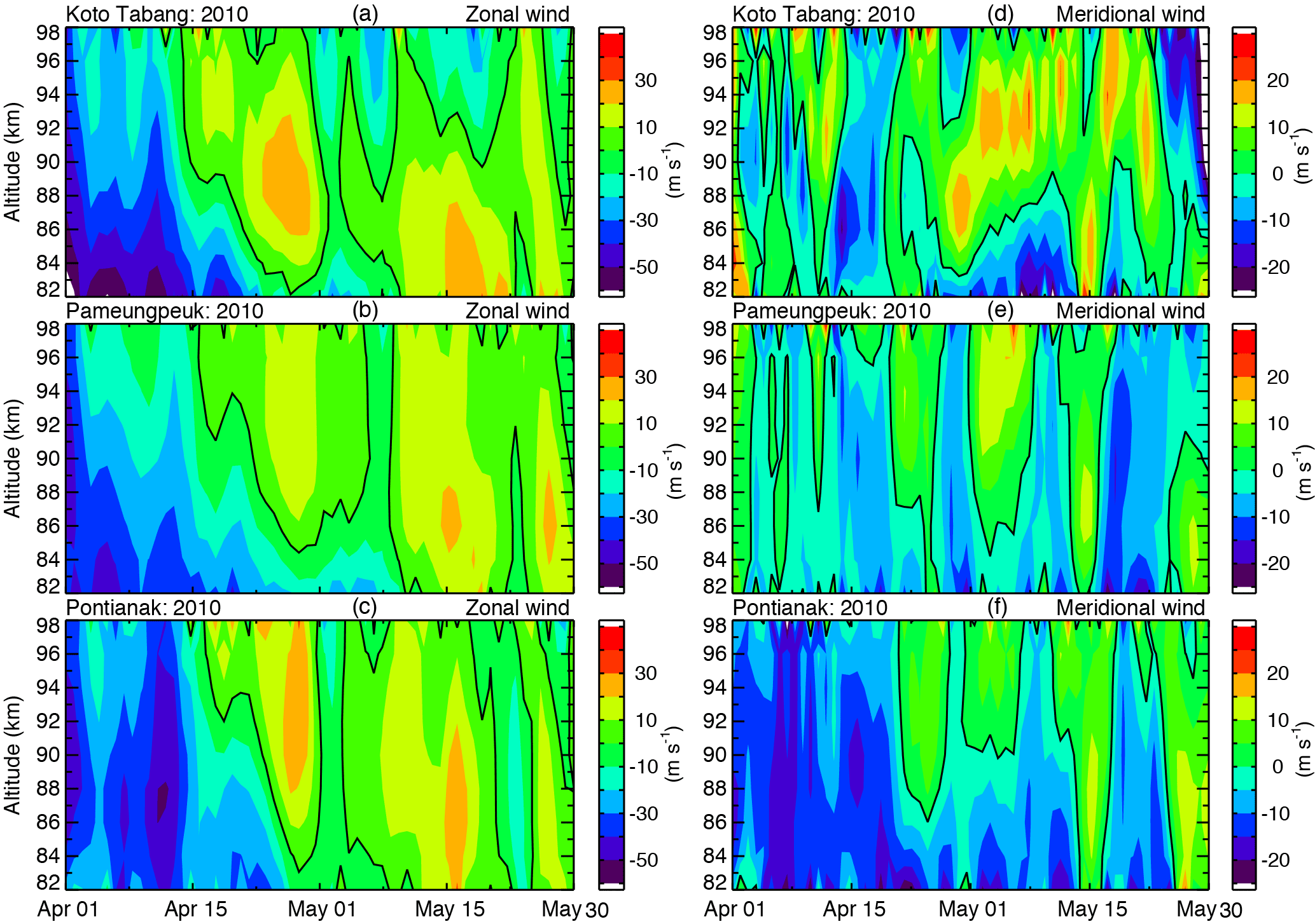
Figure 1Time–altitude sections of the daily mean zonal (a, b, c) and meridional (d, e, f) winds over Kototabang, Pameungpeuk, and Pontianak locations during the period from 1 April to 31 May 2010.
Hourly winds were used for this analysis. We examined the datasets, found small data gaps, and these data gaps were filled by linear interpolation. We applied a conventional cross-spectral (CCS) analysis technique enabling the combination of any two signals (two series) to be analyzed simultaneously. This allows us to examine the characteristics of these series and coherence of the datasets (Stoica and Moses, 2004; Bloomfield, 2005). In this spectral technique, the total power is distributed in the frequency domain. We detect periodic components in the observed signal in the time domain as demonstrated by van Hoek et al. (2016). The peaks of the spectra identify the relative importance of different frequency bands in the time domain. To examine the PWs in the middle atmosphere, a relatively new adaptive signal processing method called empirical mode decomposition (EMD), introduced by Huang et al. (1998), was used. This adaptive approach is derived from the simple assumption that any signal can be composed of different intrinsic mode functions (IMFs), each representing an embedded characteristic oscillation of a specific timescale (Huang et al., 2012). Adding all IMFs together with EMD residue will reconstruct the original signal without any loss of information or distortion. Higher frequency oscillations are captured in the first mode and subsequent modes have lower average frequencies. The first (principal) mode captures the higher frequency oscillations, with the following modes capturing successively lower frequencies. A more detailed description and methodology of extracting IMFs from the time series data can be found elsewhere (Kishore et al., 2012; Huang et al., 2012). In addition, the Lomb–Scargle periodogram (LSP) analysis method (Scargle, 1982) of spectral analysis was used for determination of PW amplitude and phase. This technique allows for the estimation of amplitude or power spectra of a time series that is unevenly spaced (Press et al., 1992). LSP weighs the data by each point rather than by each time interval. The LSP technique provides as estimate of the significance of each frequency by examining the probability of its emergence from random fluctuations (Namboothiri et al., 2002).
A band-pass filter is used in the time domain to identify possible PWs, following Kishore et al. (2005). To reduce the effect of long-term trends, all the data are detrended by a second order polynomial fit before filtering and performing the spectral analysis (Kishore et al., 2005). Here we use another adaptive spectral analysis method based on Morlet wavelets. The wavelet transform is a localized transform in both space (time) and frequency. We extract the spectral intensity from a temporally evolving signal with inherent variable frequencies (Kumar and Foufoula-Georgiou, 1997). The time-frequency resolution of a wavelet is not constant, but varies with frequency.
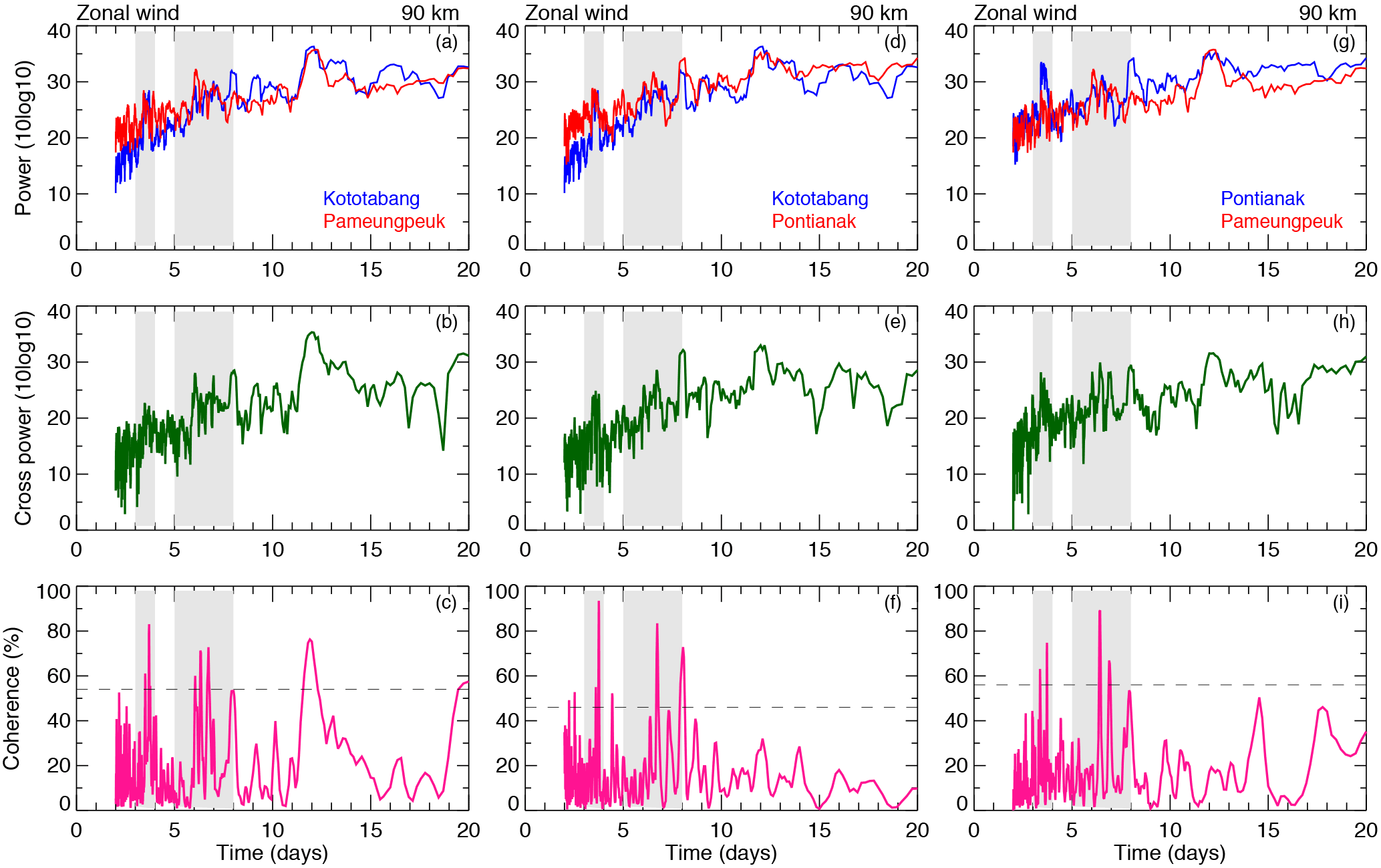
Figure 2The zonal wind power spectral density of two radars (a, d, g), cross power spectral density (b, e, h), and coherence (c, f, i) during 1 April to 31 May 2010.
3.1 Temporal variability in mean winds
In this section, we present mean wind circulation in the MLT region over the three radars located at KOT, PAM, and PON. Figure 1 illustrates the time–height plots representing the zonal winds (panels a–c) and meridional winds (panels d–f) over the altitude region of 82–94 km from 1 April to 31 May 2010. Wind contours are constructed from daily mean values, with the solid black line representing the zero wind in zonal and meridional contours. It can be seen that before mid-April, zonal winds are mostly westward for all radars, while the flow is eastward for most observation days after this period. According to Venkateswara Rao et al. (2012), westward winds are stronger than eastward winds within ±9∘ latitude, whereas at ±22∘ eastward winds are stronger. The maximum westward wind is observed to be about 40 m s−1 over KOT at an altitude of 82 km. The maximum eastward wind is in the range of ∼ 25 m s−1 and its occurrence is at around 88, 86, and 94 km over KOT, PAM, and PON, respectively. In general, a similar behavior in the zonal winds is found among the stations, and strong westward winds centered on April 2010 weaken with increasing height. Younger and Mitchell (2006) have shown that westward winds observed during the equinoxes have a maximum of about 30 m s−1, and are located at about 84 km at the Ascension Island equatorial station. The UARS High-Resolution Doppler Imager (HRDI) has also documented the tendency of the speed of westward winds (e.g., Burrage et al., 1996). Figure 1d–f represent the meridional wind for the three radar stations. The major structures produced by the three stations are generally the same. In all three stations southward wind is larger than the northward wind. The maximum southward wind is observed in early April between the 82 and 86 km altitude regions at about ∼ 25 m s−1 over PON. The maximum northward wind is observed over KOT at about ∼ 15 m s−1 between the altitudes of 86 to 92 km. Independent observations of equatorial mean winds at Ascension Island (Hirota, 1978) and other longitudes (Burrage et al., 1996) agree with the general form of the winds. These studies demonstrated that westward winds peak during the equinox while eastward winds peak during the solstice.
A cross-correlation analysis was performed between the three zonal and meridional time series between 82 and 94 km altitudes. This analysis provides a set of time-dependent correlation coefficients of two signals. We found correlation coefficients of 0.68 between KOT and PAM with a lag of zero, 0.65 between KOT and PON, and 0.63 between PON and PAM zonal wind at 86 km, which are significant at the 95 % confidence level. The maximum lag is observed in the altitude range between 90 and 94 km. In the case of meridional wind we observed a time lag of ±5 h. Figures 2 and 3 show the results of the cross-spectral analysis for the zonal and meridional winds. In Fig. 2, the top row (panels a, d, and g) shows the power spectral density of two radars, the middle row (panels b, e, and h) corresponds to the cross-spectral power, and the bottom row (panels c, f, and i) is the coherence spectrum estimated for the 90 km altitude level using the CCS technique. The dashed line in the bottom panels corresponds to the 95 % confidence level. From the figures it can clearly be seen that the zonal and meridional wind power spectra are characterized by a dominant peak at 3–4 and 5–8 days. Furthermore, these peaks appear at all mesospheric heights (82–94 km). Comparing the bottom panels of Figs. 2 and 3 demonstrates that PWs appear in the three radar datasets, and these waves are above the 95 % confidence level. The average coherence is 0.53 between the radars zonal winds and 0.5 between the meridional winds. These coherence plots identify cycles of 3–4 and 5–8 days. In addition, some other PWs (8 and 10–12 days) are also clearly evident; however, they are out of the scope of the present study.
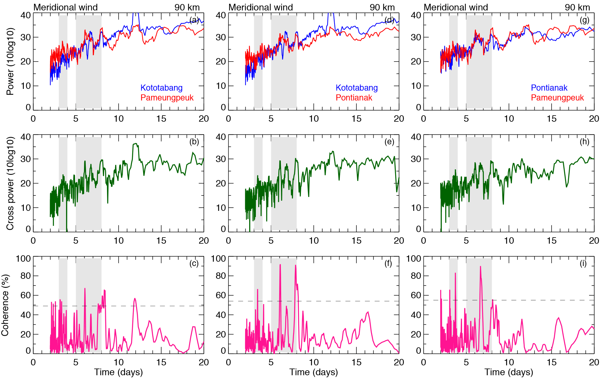
Figure 3The meridional wind power spectral density of two radars (a, d, g), cross power spectral density (b, e, h), and coherence (c, f, i) during 1 April to 31 May 2010.

Figure 4Time series of (a) daily mean zonal wind observed using the Kototabang radar during 1 to 21 May 2010 at the 90 km altitude level. Intrinsic mode function components from the first to eighth IMFs are shown in (b–i). Corresponding LSP are shown in (j–r), respectively. The dashed horizontal lines in (j–r) indicate the 95 % confidence level.
Before studying the characteristics of PWs, we checked what periods were dominant in the hourly wind datasets. We used LSP and the new analysis technique of EMD, which is an effective method for adaptively decomposing the signal into different independent frequency components, termed IMFs. The IMFs yield instantaneous frequencies as a function of time, which allows for a precise identification of embedded structures. The time series of hourly zonal wind data at 90 km altitude are shown in Fig. 4 (top left); 10 IMFs can be extracted over KOT, only 8 of which are shown here to characterize the most important components. We investigate the gross characteristics of oscillations for each IMF using LSP analysis to the IMF time series. All IMFs exhibit slow-varying amplitudes and frequencies. The amplitude spectral plots are shown in the right panels of Fig. 4. The 95 % confidence level is shown by a horizontal dashed line. For this figure, the selected altitude is 90 km from the KOT hourly zonal wind dataset. The figure shows that the dominant peaks near semi-diurnal (12 h) and diurnal (24 h) are present in IMF2 and IMF4. IMF7 shows a clear PW period of about 3.5 days, while IMF8 shows a broader range of oscillations with periods ranging from 5 to 8 days and the maximum amplitude occurring at about 6.5 days. The Lomb–Scargle amplitude spectra are shown on the right side of Fig. 4, which reveals components centered at ∼ 3.6 and 6.5 days. The 3.6-day peak is somewhat broad, extending over roughly 3–5 days. Similarly, the 6.5-day wave also shows a broad peak (∼ 5–8.0 days). The EMD technique reveals that some waves with periods that are close to those of diurnal tide are generated due to the interactions of the diurnal tide and PWs, which indicate extensive coupling between the diurnal tide and PWs (Takahashi et al., 2006). In both methods, the PWs in mesospheric altitudes over equatorial radars are clearly seen. The PW periods are observed throughout mesospheric altitudes at all stations, although their amplitudes vary with altitude and from station to station. Similar results are also found at the other radars, indicating that these IMFs are statistically different from noise.
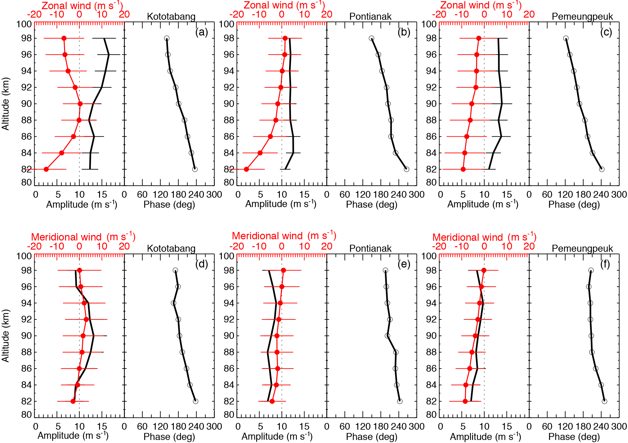
Figure 5Height profiles of the amplitudes and phases (open circle) of the 3.6-day waves over Kototabang, Pameungpeuk, and Pontianak locations. The thick solid lines represent the mean zonal winds over the period from 1 April to 31 May 2010.
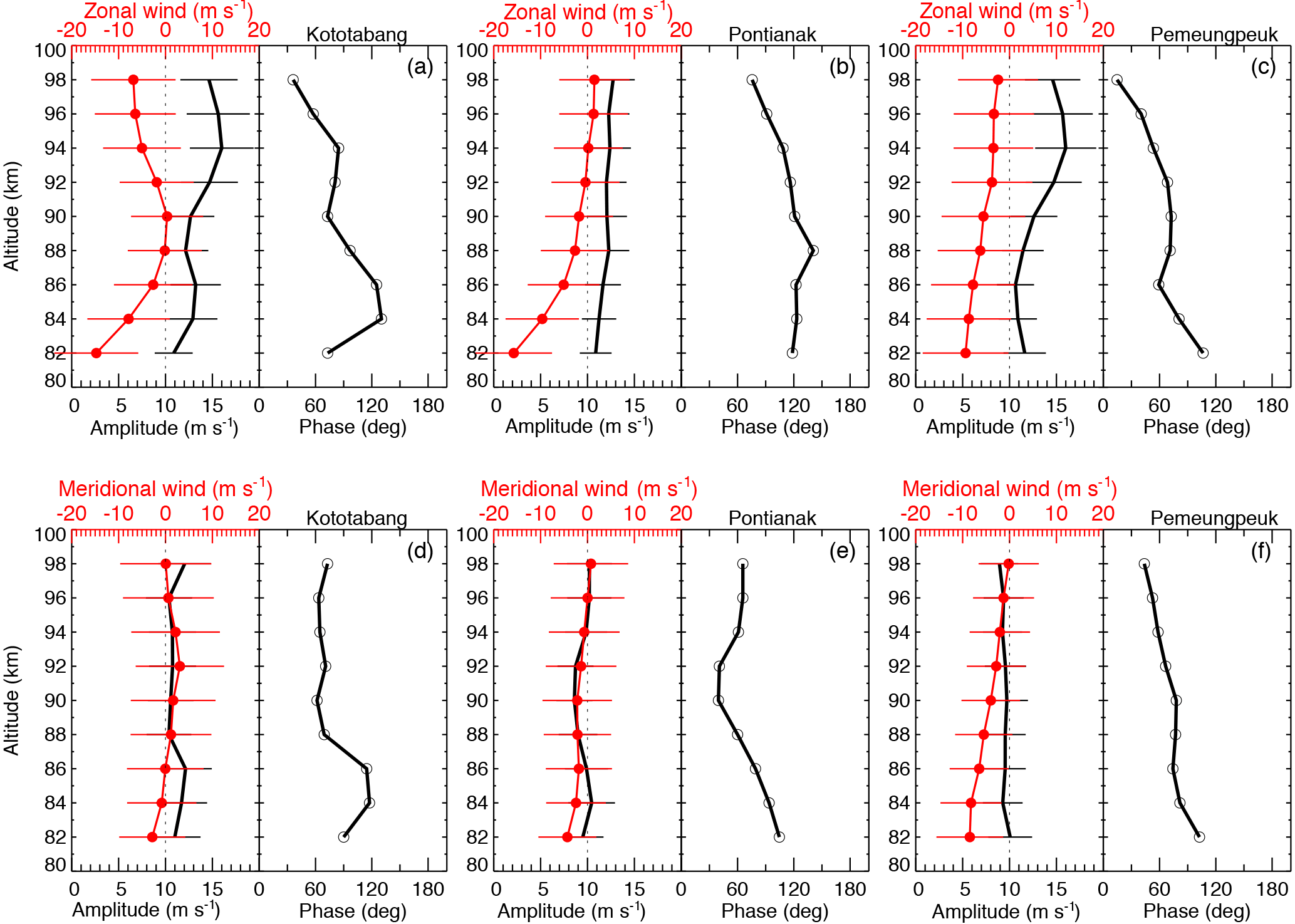
Figure 6Height profiles of the amplitudes and phases (open circle) of the 6.5-day waves over Kototabang, Pameungpeuk, and Pontianak locations. The thick solid lines represent the mean zonal winds over the period from 1 April to 31 May 2010.
To deduce more information on the dependence of the PWs on height variations in Figs. 5 and 6, we show the mean wind, amplitudes, and phases over the three stations for the observation period. In each figure the top and bottom panels represent the zonal and meridional winds, respectively, as well as the amplitude and phase profiles for each station. The spectral amplitudes and phases were calculated by a LSP analysis within a set time window of 14 days (26 days) in length for the 3.6-day (6.5-day) wave. This window was shifted by a step size of 1 day, and the power spectral amplitude and phase values were estimated. The amplitude and corresponding phase values were considered only when they are > 95 % significant. Mean zonal and meridional winds are also given (curves with solid curves) to show the response of the PWs to background winds. Generally speaking, the 3.6-day zonal amplitudes look similar in all three stations. For example, at KOT and PAM the peaks are as large as 12–14 m s−1 above 90 km. But at Pontianak the zonal 3.6-day amplitudes are smaller and have no prominent peak values. When comparing the 3.6-day wave amplitude with background zonal mean wind, it seems that when there is a westward wind flow, there is also stronger 3.6-day amplitudes. The phase profiles (solid curves with open circles) indicate fairly downward progression in the 82–94 km height range at almost all three stations. KOT, PAM, and PON have vertical wavelengths of 42, 44, and 40 km, respectively. Note that these values are close to those estimated for equatorial regions and the vertical wavelengths are slightly smaller than the theoretical estimates for a 3.6-day wave.
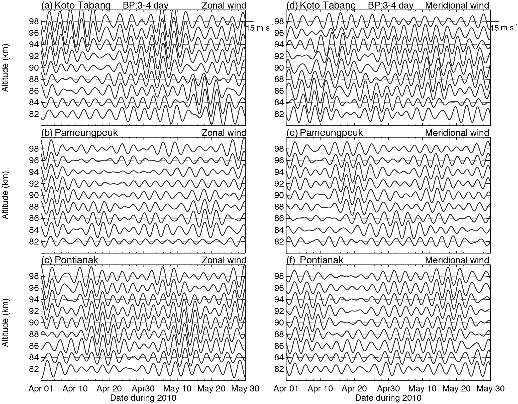
Figure 7The band-pass filter results of the zonal (a, b, c) and meridional (d, e, f) at Kototabang, Pameungpeuk, and Pontianak locations. The bandwidth is 3–4 days and the interval is 15 m s−1.
Figure 6 shows the mean vertical profiles of the 6.5-day wave amplitudes and phases observed in the zonal (top panels) and meridional (bottom panels) wind components at the three equatorial stations, together with the mean wind. In the figure, the 6.5-day wave amplitude is shown by solid curves, mean wind is shown by curves with solid circles, and the phase is indicated by curves with open circles. The amplitudes are generally < 10 m s−1 below 90 km altitude levels. The maximum amplitudes (12–14 m s−1) are observed at KOT and PAM radar stations at 94 km of altitude, while moderate amplitudes are observed over the PON radar. Jiang et al. (2008) observed that 6.5-day wave amplitudes were strongest between 84 and 98 km, and the maximum amplitude of ∼ 14.5 m s−1 appeared at 92 km in April–May 2004 using the Wuhan meteor radar. Furthermore, they indicated that the 6.5-day waves near the spring equinox were generally stronger than those in other seasons. A large mesospheric 6.5-day wave was seen during late April and early May 2003 by the SABER instrument aboard the TIMED satellite and the ground-based radar systems (Riggin et al., 2006; Jiang et al., 2008). They mentioned that the 6.5-day wave in the MLT region during April–May 2003 should be regarded as an atmospheric normal mode, which was amplified through sympathetic interaction with the background wind. Takahashi et al. (2006) reported observations of a very strong ∼ 6-day wave with amplitudes reaching ∼ 25 m s−1 present simultaneously in the zonal winds over Cariri (7.4∘ S) and Ascension Island (7.9∘ S). Liu et al. (2004) using the National Center for Atmospheric Research Thermosphere-Ionosphere-Mesosphere Electrodynamics General Circulation Model (TIME-GCM) investigated the structures and seasonal variability in 6.5-day waves. The phase profiles of the 6.5-day wave for zonal and meridional winds for the three radars are shown adjacent to the wind profiles in Fig. 6. Usually there is a downward propagation with time, although upward phase progressions are sometimes observed.
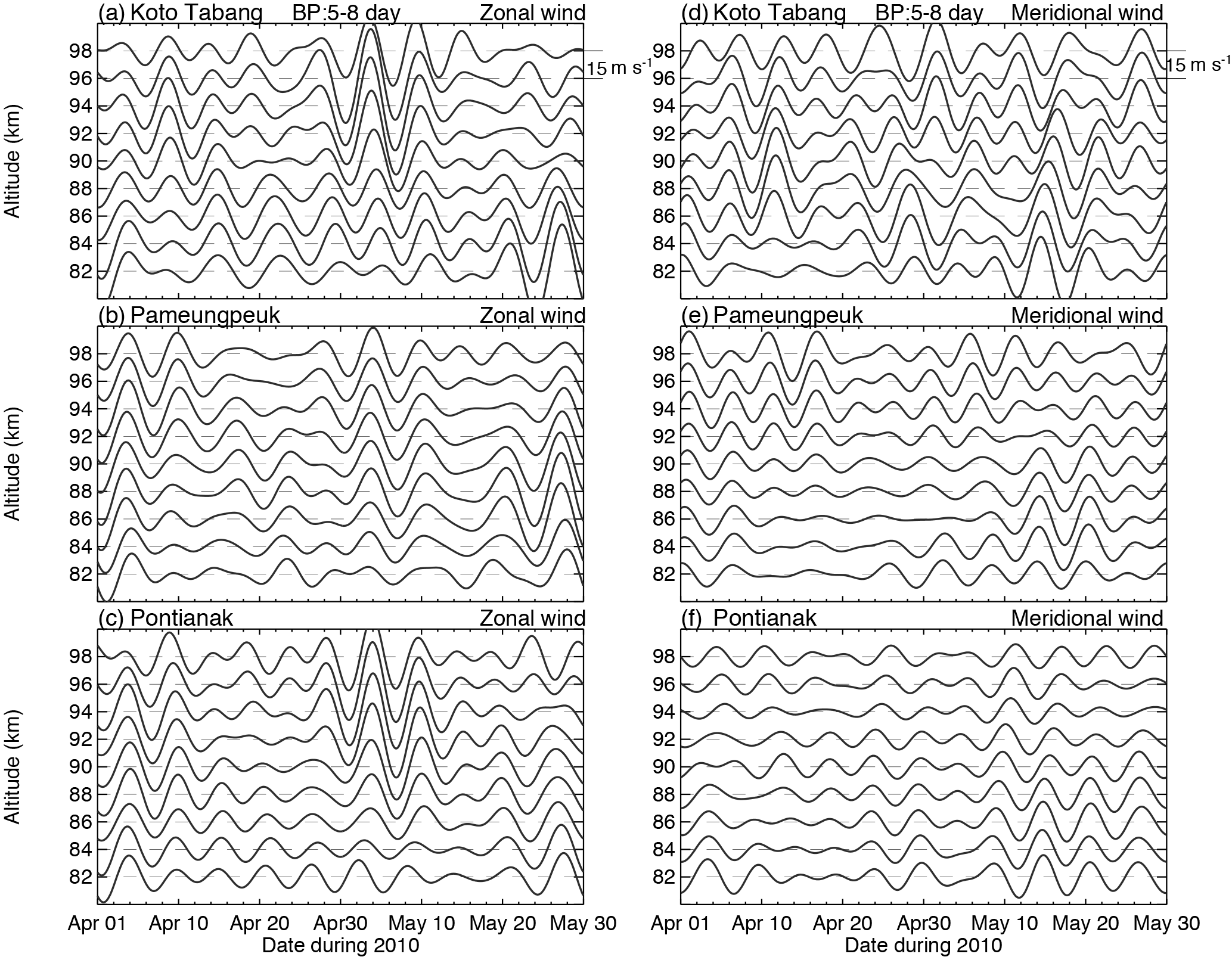
Figure 8The band-pass filter results of the zonal (a, b, c) and meridional (d, e, f) winds at Kototabang, Pameungpeuk, and Pontianak. The bandwidth is 5–8 days and the interval is 15 m s−1.
In order to further investigate these waves, a band-pass filtering analysis of the horizontal winds in each height grid was carried out. The dominance of the 3.6-day wave periodicity is also clearly evident in the filtered time series of all three radars as shown in Fig. 7. In this figure, we considered step sizes of 2 km between the heights of 82 and 94 km. The data at the three sites were subjected to an elliptical band-pass filter with cutoff periods of 3.0–4.0 days. The figure clearly shows the time variations in the occurrence of the 3.6-day wave, with the KOT amplitudes being larger than those of the other two radars. The largest wave activity, with amplitudes of ∼ 16 m s−1, occurred at 92 km in the zonal wind during 1–15 April and 20 April–10 May over KOT. While the zonal and meridional wind components have similar amplitudes near the equator, the zonal 3.6-day wave amplitudes are larger than the meridional wind amplitudes. This is consistent with the other measurements.
Next, we perform a similar analysis with the 6.5-day oscillations. Figure 8 illustrates the features of the 6.5-day oscillations at different heights from 82 to 94 km. The zonal and meridional wind dataset was subjected to a band-pass filter of 5–8 days width. The amplitude of the oscillations at KOT reached ∼ 16 m s−1 at 88–94 km and lasted for 2 to 3 cycles in the 21-day interval spanning 22 April to 12 May 2010. It is interesting to note that the 6.5-day zonal wind oscillations at KOT, PAM, and PON were almost in phase during this period. The PAM and PON zonal winds showed common oscillation features during the intervals 1–14 April and 20 April–12 May 2010. The KOT zonal wind showed larger amplitudes than the other equatorial sites. The filter analysis determined that 6.5-day waves have a period of about 6–7.5 days, with the maximum wave amplitude occurring at 6.5 days. The zonal 6.5-day amplitudes are generally slightly stronger than the meridional amplitudes in all radar observations.
3.2 Wavelet analysis of the 3.6- and 6.5-day oscillation variability
In this section, we investigate the possible temporal modulation of 3.6 and 6.5-day waves throughout the observation period through wavelet analysis. Figures 9 and 10 show the 3.6 and 6.5-day periodicities at three different height levels (86, 90, and 94 km) over three different radars. Wavelet analysis was applied to the dataset for the period 1 April–31 May 2010 for constructing the contours. Specifically, the commonly used Morlet wavelet function was used which better captures the time-varying nature periodicities. The details of this method can be found in Torrence and Compo (1998). In the figures, the 3.6- and 6.5-day periods are marked by white dotted lines.
In Fig. 9 we illustrate the 3.6-day zonal spectral intensities observed at 86, 90, and 94 km for the three radars. It is evident that during the observation period, a large burst of wave activity with a period of about 3.6 days occurred at all altitude levels. The wave period extended 2–5 days but the maximum intensity was near 3.6 days. The black line in the plots indicates areas with 95 % confidence level. The white dotted line indicates the 3.6-day wave period. From the figure, the wave intensity at higher altitudes appears to be slightly larger than that at the lower altitude levels. Figure 9d shows wider periods oscillating at 2–7 day periods. The 3.6-day wave amplitudes at PON have slightly smaller amplitudes compared to the other two radars.
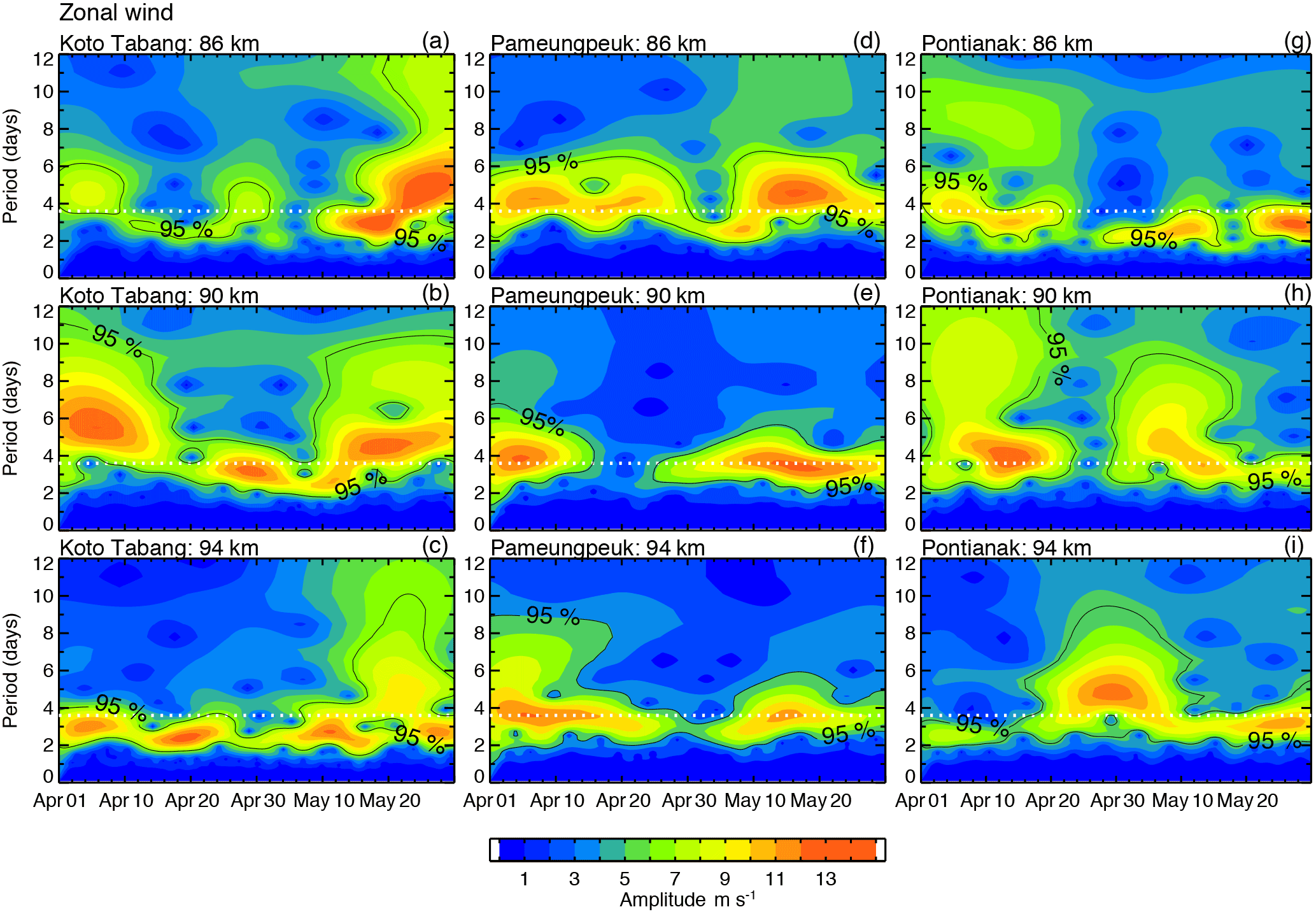
Figure 9Contours of wavelet intensities as a function of frequency and time for the zonal wind of IMF3 at three different heights (86, 90, and 94 km) over Kototabang, Pameungpeuk, and Pontianak locations.

Figure 10Contours of wavelet intensities as a function of frequency and time for the zonal wind of IMF5 at three different heights (86, 90, and 94 km) over Kototabang, Pameungpeuk, and Pontianak locations.
To deduce more information on the time–height variations and dependence of the 6.5-day wave, we show the amplitudes at the three radars at 86, 90, and 94 km in Fig. 10. The 6.5-day peak is somewhat broad, ranging over 5–8 days at some heights and 5–10 days at other levels. The wave amplitude increases with altitude and reaches a maximum of about 22 K at mesospheric altitudes for all three radars. The 6.5-day oscillation has a broad spectral peak extending over several days at 90 and 94 km of altitude at KOT. The maximum amplitude of ∼ 24 K is observed over KOT at altitudes of around 94 km. The temporal localization oscillations using wavelet analysis shows strong 6.5-day waves during the observation period. During the observation period, the maximum amplitudes show differences between the measurements and thus make the wave activity out of phase at these locations (Kishore et al., 2005).
In the present study we made an attempt to study the planetary wave (PW; 3.6- and 6.5-day) oscillations over three radars (KOT, PAM, and PON) installed in tropical latitudes during the period from 1 April to 31 May 2010. The main findings obtained from this study are summarized below:
The major zonal wind structures produced by the three stations are generally the same. The main features of the zonal winds are mostly westward before mid-April, and thereafter eastward wind is observed in all three radar stations. The maximum westward wind seems similar in all three stations, while the maximum westward jet is observed at different altitudes at each station. The maximum southward wind is observed in early April between the 82 and 94 km altitude levels in all three radars. Furthermore the southward wind is stronger than the northward wind.
Empirical mode decomposition (EMD) is a novel method to extract time-varying quantities from time series of data. This method decomposes a time series into intrinsic oscillations using the local temporal structural characteristics of the data. Each consequent IMF is a narrowband time series with an identifiable central period around which the oscillations take place. The analysis revealed strong signatures of 3.5- and 6.5-day waves. The EMD also showed higher frequencies of 12 and 24 h, as well as 2–2.5 days. The EMD technique was used to explore planetary waves over three equatorial radars.
The 3.6-day wave amplitudes were somewhat similar across all the radars, with the maximum mean amplitude observed in KOT and PAM at ∼ 12 m s−1, always above the 90 km altitude level. The phase profiles showed a fairly downward progression, with an estimated mean vertical wavelength of about 42 km.
The amplitudes of the 6.5-day waves show roughly similar values in all three radars. However, the zonal amplitude reaches its maximum at altitudes between 90 and 94 km with a peak value of ∼ 12 m s−1 in KOT and PAM radars. The PON zonal 6.5-day amplitudes are slightly smaller compared to the other two radars. Vertical wavelengths are observed to be between 30 and 38 km with the network of the three radars, which is similar to the equatorial site measurements.
To understand the temporal behavior of the PW (3.6- and 6.5-day) oscillations, we used a wavelet transform technique at three different altitudes for the network of radars. Furthermore, it suggested that these oscillations are dominant in the mesosphere over equatorial regions. In a future study we will combine datasets from other equatorial stations with long-term observations, which will allow for a better understanding of wave characteristics and including the wave number.
Data can be provided on request to Atsuki Shinbori, Research Institute for Sustainable Humanosphere (RISH), Kyoto University, Japan.
The authors declare that they have no conflict of interest.
We would like to thank the Research Institute for Sustainable Humanosphere
(RISH), Kyoto University and all associated members involved in data
acquisition by the network of radars. Distribution of the data has been
partly supported by the Inter-university Upper atmosphere Global Observation
NETwork (IUGONET) project funded by the Ministry of Education, Culture,
Sports, Science and Technology (NEXT), Japan. Gummadipudi Nagasai Madhavi is
grateful to the Department of Science and Technology (DST-SERB) for providing
the National Post-Doctoral Fellowship.
The topical editor, Andrew J.
Kavanagh, thanks Quan Gan and one anonymous referee for help in evaluating
this paper.
Briggs, B. H.: The analysis of spaced sensor records, in: Handbook for Map, edited by: Vincent, R. A., 13, 166–186, 1984.
Bloomfield, P.: The spectrum, in: Fourier analysis of time series, John Wiley and Sons, New York, NY, USA, 133–166, 2005.
Burrage, M. D., Vincent, R. A., Mayr, H. G., Skinner, W. R., Arnold, N. F., and Hays, P. B.: Long-term variability in the equatorial middle atmosphere zonal wind, J. Geophys. Res., 101, 12847–12854, https://doi.org/10.1029/96JD00575, 1996.
Charney, J. G. and Drazin, P. G.: Propagation of planetary scale disturbances from the lower to the upper atmosphere, J. Geophys. Res., 66, 83–109, 1961.
Clark, R. R., Burrage, M. D., Franke, S. J., Manson, A. H., Meek, C. E., Mitchell, N. J., and Muller, H. G.: Observations of 7-d planetary waves with MLT radars and the UARS-HRDI instrument, J. Atmos. Sol.-Terr. Phy., 64, 1217–1228, 2002.
Dhanya, R., Gurubaran, S., and Emperumal, K.: Lower E-region echoes over the magnetic equator as observed by the MF radar at Tirunelveli (8.7∘ N, 77.8∘ E) and their relationship to Esq and Esb, Ann. Geophys., 26, 2459–2470, https://doi.org/10.5194/angeo-26-2459-2008, 2008.
Forbes, J. M.: Wave coupling between the lower and upper atmosphere: case study of an ultra-fast Kelvin wave, J. Atmos. Sol.-Terr. Phy., 62, 1603–1621, 2000.
Garcia, R. R., Lienerman, R., Russell III, J. M., and Mlynczak, M. G.: Large-scale waves in the mesosphere and lower thermosphere observed by SABER, J. Atmos. Sci., 62, 4384–4399, 2005.
Gregory, J. B., Meek, C. E., and Manson, A. H.: An assessment of winds data (60–110 km) obtained in real-time from a medium frequency radar using the radio wave drifts technique, J. Atmos. Sol.-Terr. Phy., 44, 649–655, 1982.
Hirota, I.: Equatorial waves in the upper stratosphere and mesosphere in relation to the semiannual oscillation of the zonal wind, J. Atmos. Sci., 35, 714–722, 1978.
Holton, J.: Waves in the equatorial stratospheric generated by tropospheric heat resources, J. Atmos. Sci., 27, 368–375, 1972.
Holton, I.: Kelvin waves in the equatorial middle atmosphere observed by the Nimbus 5 SCR, J. Atmos. Sci., 36, 217–222, 1979.
Huang, B., Hu, Z. Z., Kinter, J. L., Wu, Z., and Kumar, A.: Connection of stratospheric QBO with global atmospheric general circulation and tropical SST. Part 1: methodology and composite life cycle, Clim. Dynam., 38, 1–23, 2012.
Huang, N. E., Shen, Z., Long, S. R., Wu, M. C., Shih, H. H., Zheng, Q., Yen, N. C., Tung, C. C., and Liu, H. H.: The empirical mode decomposition and the Hilbert spectrum for nonlinear and non-stationary time series analysis, P. Roy. Soc. Lond. A Mat., 454, 903–995, 1998.
Jiang, G., Xu, J., Xiong, J., Ma, R., Ning, B., Murayama, Y., Thorsen, D., Gurubaran, S., Vincent, R. A., Reid, I., and Franke, S. J.: A case study of the mesospheric 6.5-day wave observed by radar systems, J. Geophys. Res., 113, D16111, https://doi.org/10.1029/2008JD009907, 2008.
Kishore, P., Namboothiri, S. P., Igarashi, K., Gurubaran, S., Sridhran, S., Rajaram, R., and Venkat Ratnam, M.: MF radar observations of 6.5-day wave in the equatorial mesosphere and lower thermosphere, J. Atmos. Sol.-Terr. Phy., 66, 507–515, 2004.
Kishore, P., Subba Reddy, I. V., Namboothiri, S. P., Igarashi, K., Venkat Ratnam, M., Narayana Rao, D., and Vijaya Bhaskara Rao, S.: Study of equatorial Kelvin waves using the MST radar and radiosonde observations, Ann. Geophys., 23, 1123–1130, https://doi.org/10.5194/angeo-23-1123-2005, 2005.
Kishore, P., Velicogna, I., Venkat Ratnam, M., Jiang, J. H., and Madhavi, G. N.: Planetary waves in the upper stratosphere and lower mesosphere during 2009 Arctic major stratospheric warming, Ann. Geophys., 30, 1529–1538, https://doi.org/10.5194/angeo-30-1529-2012, 2012.
Kumar, P. and Foufoula-Georgiou, E.: Wavelet analysis for geophysical applications, Rev. Geophys., 35, 385–412, 1997.
Liu, H. L., Tallat, E. R., Roble, R. G., Liberman, R. S., Riggin, D. M., and Yee, J. H.: The 6.5-day wave and its seasonal variability in the middle and upper atmosphere, J. Geophys. Res., 109, D21112, https://doi.org/10.1029/2004JD004795, 2004.
Meyer, C. K. and Forbes, J. M.: A 6.5-day westward propagating planetary wave: Origin and its characteristics, J. Geophys. Res., 102, 26173–26178, 1997.
Namboothiri, S. P., Kishore, P., and Igarashi, K.: Climatological studies of the quasi 16-day oscillations in the mesosphere and lower thermosphere at Yamagawa (31.2∘ N, 130.6∘ E), Japan, Ann. Geophys., 20, 1239–1246, https://doi.org/10.5194/angeo-20-1239-2002, 2002.
Pancheva, D., Mitchell, N. J., and Younger, P. T.: Meteor radar observations of atmospheric waves in the equatorial mesosphere/lower thermosphere over Ascension Island, Ann. Geophys., 22, 387–404, https://doi.org/10.5194/angeo-22-387-2004, 2004.
Pancheva, D., Mukhtarov, P., Andonov, B., and Forbes, J. M.: Global distribution and climatological features of 5–6 day planetary waves seen in the SABER/TIMED temperatures (2002–2007), J. Atmos. Terr. Phys., 72, 26–37, https://doi.org/10.1016/J.jastp.2009.10.005, 2010.
Press, W. H., Teukolsky, S. A., Vetterling, W. T., and Flannery, B. P.: Numerical Recipes in C, Cambridge University Press, New York, 2002.
Ramkumar, T. K., Gurubaran, S., and Rajaraman, R.: Lower E-region MF radar spaced antenna measurements over magnetic equator, J. Atmos. Sol.-Terr. Phy., 64, 1445–1453, 2002.
Riggin, D. M., Fritts, D. C., Tsuda, T., Nakamura, T., and Vincent, R. A.: Radar observations of 1 3-day Kelvin wave in the equatorial mesosphere, J. Geophys. Res., 102, 26241–26157, 1997.
Riggin, D. M. Liu, H., Lieberman, R. S., Robble, R. G., Russell III, J. M., Mertens, C. J., Mlynczak, M. G., Pancheva, D., Franke, S. J., Murayama, Y., Manson, A. H., Meek, C. E., and Vincent, R. A.: Observations of the 5-day wave in the mesosphere and lower thermosphere. J. Atmos. Sol.-Terr. Phy., 68, 323–339, https://doi.org/10.1016/j.jastp.2005.05.010, 2006.
Salby, M. and Garcia, R.: Transient response to localized episodic heating in the tropics, Part 1: excitation and short-time near-field behavior, J. Atmos. Sci., 44, 458–498, 1987.
Salby, M. L., Hartmann, D. L., Bailey, P. L., and Gille, J. C.: Evidence for equatorial Kelvin modes in Nimbus-7 LIMS, J. Atmos. Sci., 41, 220–235, 1984.
Scargle, J. D.: Studies in astronomical time series analysis. II, Statistical aspects of spectral analysis of unevenly spaced data, J. Astrophys., 263, 835–853, 1982.
Stoica, P. and Moses, R. I.: Spectral analysis of Signals, Prentice Hall, Bergen, NJ, USA, 2004.
Takahashi, H., Wrasse, C. M., Pancheva, D., Abdu, M. A., Batista, I. S., Lima, L. M., Batista, P. P., Clemesha, B. R., and Shiokawa, K.: Signatures of 3–6 day planetary waves in the equatorial mesosphere and ionosphere, Ann. Geophys., 24, 3343–3350, https://doi.org/10.5194/angeo-24-3343-2006, 2006.
Takahashi, H., Wrasse, C. M., Fechine, J., Pancheva, D., Abdu, M. A., Batista, I. S., Lima, I. M., Batista, P. P., Clemesha, B. R., Schuch, N. J., Shiokawa, K., Gobbi, D., Mlynczak, M. G., and Russell, J. M.: Signatures of ultra fast Kelvin waves in the equatorial middle-atmosphere and ionosphere, Geophys. Res. Lett., 34, L11108, https://doi.org/10.1029/2007GL029612, 2007.
Talaat, E. R., Yee, J.-H., and Zhu, X.: Observations of the 6.5-day wave in the mesosphere and lower thermosphere, J. Geophys. Res., 106, 20715–20723, 2001.
Torrence, C. and Compo, G. P.: A practical guide to Wavelet Analysis, B. Am. Meteorol. Soc., 79, 61–78, 1998.
Tsuda, T., Kato, S., and Vincent, R. A.: Long period wind oscillations observed by the Kyoto meteor radar and comparison of the quasi 2-day wave with Adelaide HF radar observations, J. Atmos. Terr. Phys., 50, 225–230, 1988.
van Hoek, M., Jia, L., Zhou, J., Zheng, C., and Menenti, M.: Early drought detection by spectral analysis of satellite time series of precipitation and normalized difference vegetation index (NDVI), Remote Sens., 8, 422, https://doi.org/10.3390/rs8050422, 2016.
Venkateswara Rao, N., Tsuda, T., Gurubaran, S., Miyoshi, Y., and Fujiwara, H.: On the occurrence and variability of the terdiurnal tide in the equatorial mesosphere and lower thermosphere and a comparison with the Kyushu-GCM, J. Geophys. Res., 116, D02117, https://doi.org/10.1029/2010JD014529, 2011.
Venkateswara Rao, N., Tsuda, T., Riggin, D. M., Gurubaran, S., Reid, I. M., and Vincent, R. A.: Long-term variability of mean winds in the mesosphere and lower thermosphere at low latitudes, J. Geophys. Res., 117, A10312, https://doi.org/10.1029/2012JA017850, 2012.
Williams, C. R. and Avery, S. L.:Analysis of long-period waves using the mesosphere-stratosphere-troposphere radar at Poker Flat, Alaska, J. Geophys. Res., 97, 855–861, 1992.
Younger, P. T. and Mitchell, N. J.: Waves with period near 3 days in the equatorial mesosphere and lower thermosphere over Ascension Island, J. Atmos. Sol.-Terr. Phy., 68, 369–378, 2006.