2.1 Swarm mission and onboard GPS receivers

The Swarm constellation is composed of three identical satellites and launched on 22 November 2013 into a near-polar (87.5^∘ inclination) orbit with initial altitude of about 500 km. During the first 2 months the satellites orbited in a string-of-pearls configuration at the same altitude, and from January 2014 onward the three spacecraft were maneuvered apart and achieved their final constellation on 17 April 2014. From then on the lower pair, Swarm A and C, is flying side by side at an altitude of about 470 km, with longitudinal separation of about 1.4^∘ (about 150 km). The third spacecraft, Swarm B, orbits the Earth at about 520 km with a higher inclination (van den Ijssel et al., 2015). For covering all 24 h local times, Swarm A and C need about 133 days, while Swarm B needs about 141 days.

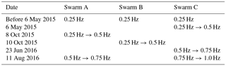
The three Swarm satellites carry dual-frequency GPS receivers of the same type, including an antenna on the topside looking upward. The receivers are equipped with eight channels to receive signals from at most eight GPS satellites simultaneously. During the past years the settings of the receivers have been updated several times. For example, the GPS observation data were first delivered with a time resolution of 10 s before 15 July 2014, and then increased to 1 s resolution afterwards; the field of view (FOV) and phase-locked loop (PLL) bandwidth have also been changed, but carried out at different dates for the three satellites. The details of the Swarm GPS receiver updates can be found in Table 1 of Van den Ijssel et al. (2016).

Table 1The increases of L2 phase-locked loop bandwidth of Swarm satellites.

Download Print Version | Download XLSX

The GPS signal is in fact affected by the ionospheric irregularities along the signal path between GPS satellite and receiver. Zakharenkova et al. (2016) has compared Swarm in situ electron density and total electron content (TEC) measurements when irregularities were observed, and their results showed quite consistent distributions between the two datasets, which also demonstrated that most of the plasma irregularities are expected in the vicinity of the altitude of Swarm satellites. Therefore, in this study we used the in situ electron density from Langmuir probes of Swarm, to check the ionospheric background conditions when signal loss happened.

2.2 GPS signal loss event detection

We used the same approach as described in Xiong et al. (2016a) for quantifying GPS signal loss events from Swarm Level-1b data (RINEX 3.00 file: GPSx_RO_1B), and the reader is referred to this paper for more details. In a nutshell, a GPS satellite associated with a certain pseudo-random noise (PRN) whose signal received by the receiver is called “in the field of view” and the GPS satellite is then called a “visible satellite”. GPS signal loss is identified as an interruption (missing epoch or data gap) of the received signal. However, we have to note that the Swarm ground processor was changed when delivering the RINEX files: before 11 April 2016 if there is an invalid value on either the L1 or L2 frequency, the epoch will not be recorded in the RINEX file; afterwards if an invalid value is only found in one of the two carrier frequencies, the epoch will still be recorded in the RINEX file but the invalid value is then written as zero. As for the kinematic precise orbit determination (POD) or TEC derivation, the phases on both L1 and L2 frequencies are needed. Therefore, for the later period we have also taken the epoch as a missing epoch if zero values are found on either frequency, and considered it as an interruption. Similar to Xiong et al. (2016a), the interruption is expected to last less than a certain period (Δt_max) before the GPS satellite becomes visible again, and we set also the Δt_max to 30 min in this study. For representing the results we took the midpoint between start and end for each signal loss event, and if two GPS signal loss events occur close to each other (less than 1 min apart), they are combined and considered as one event.

Figure 1(a) The occurrence ratio of the duration (Δt) for GPS signal loss events observed by the three Swarm satellites. The detailed occurrence ratio of events with Δt<1 min during the two periods are shown. The RINEX records time resolutions are (b) 10 s and (c) 1 s.

Download

Figure 2Global distributions of GPS signal loss events observed by three Swarm satellites.

Download

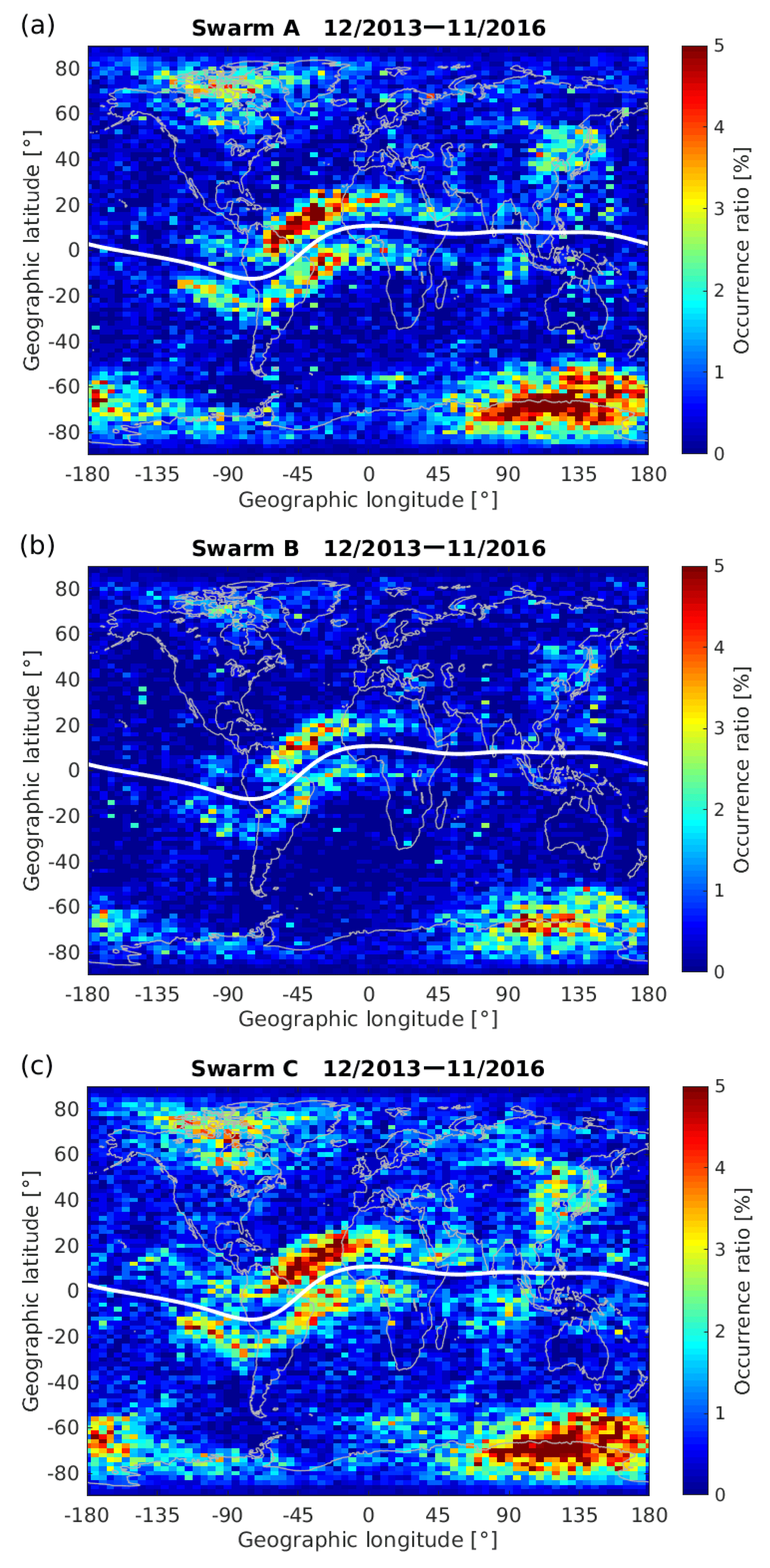
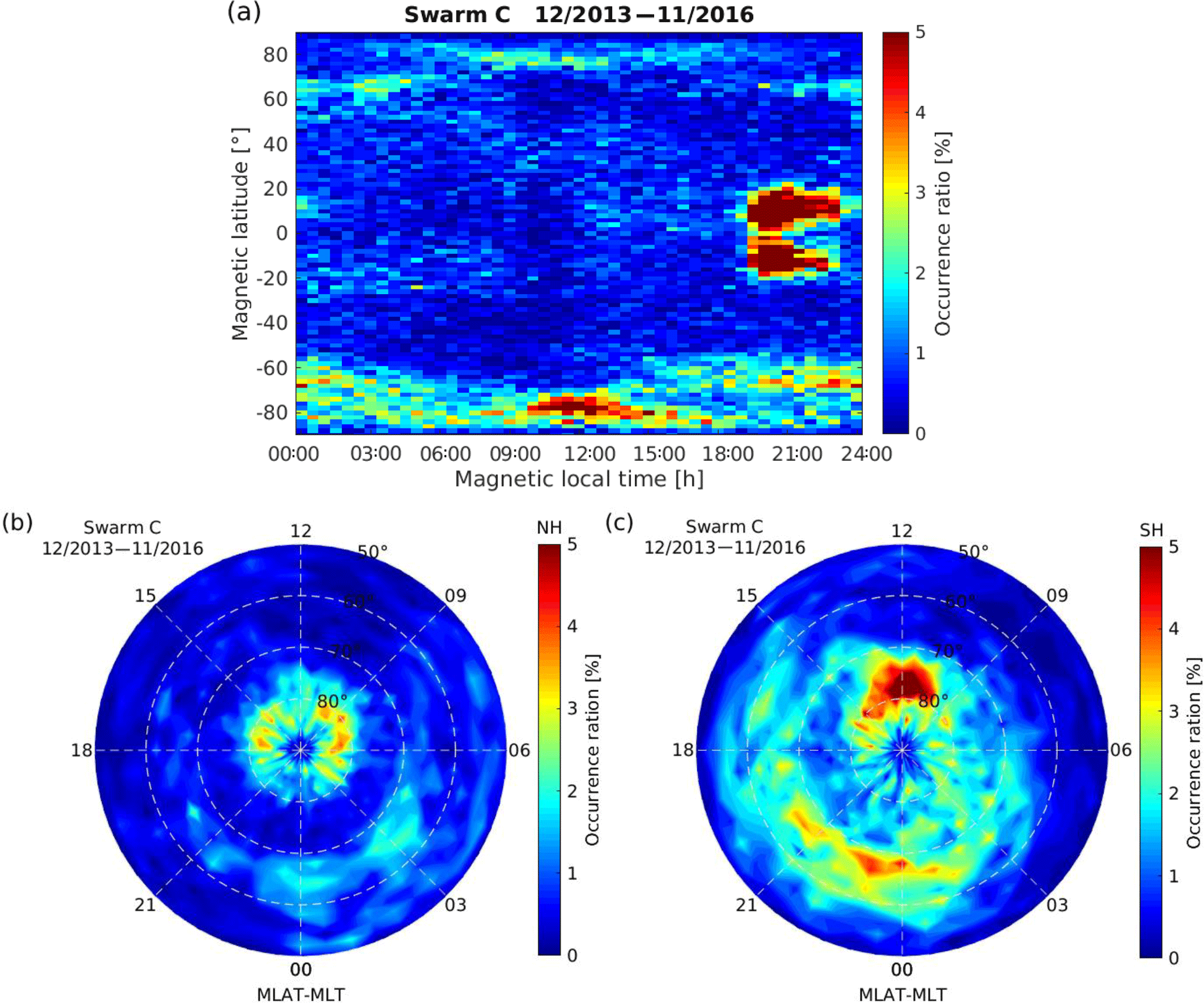
Figure 3(a) The MLAT vs. MLT distribution of GPS signal loss observed by Swarm C. (b) Similar to (a) but only for northern high latitudes (MLAT >50^∘) in the polar view. (c) Similar to (a) but for the southern high latitudes (MLAT $<-$50^∘).

Download

Figure 4(a) One example of how to determine the high-latitude plasma density gradient (ΔNe) along track from the in situ Ne measurements of Swarm C. The MLAT vs. MLT distribution of ΔNe in the (b) northern and (c) southern hemispheres, and only the passes with GPS signal loss events observed has been taken into account. (d) and (e) are similar to (b) and (c) but for the passes without GPS signal loss events.

Download

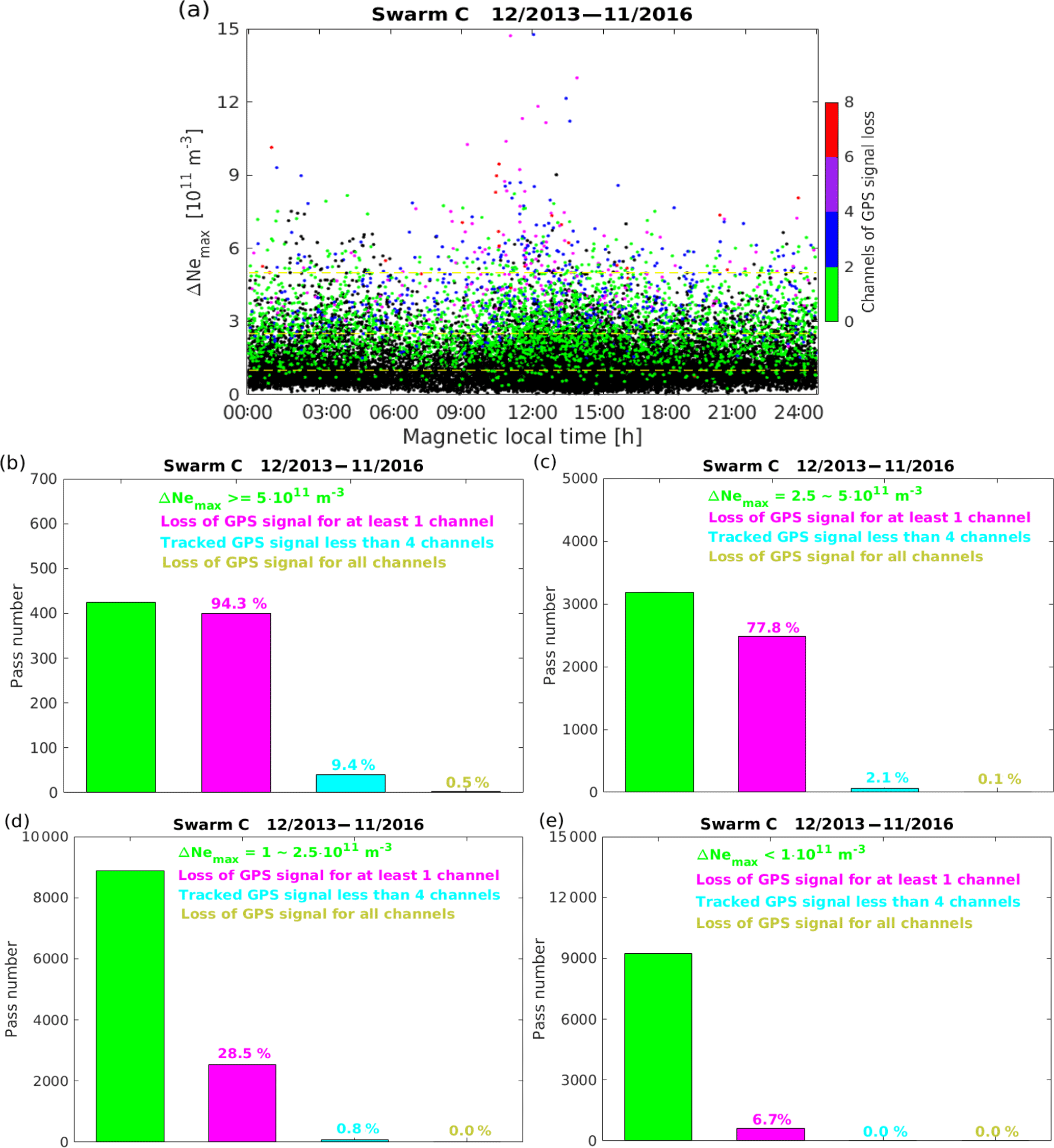
Figure 5(a) The MLT distribution of the maximum density gradients (ΔNe_max) determined from orbital arcs within $\left|\text{MLAT}\right|\ge \mathrm{50}{}^{\circ }$ and the ΔNe_max corresponds to GPS signal loss at different numbers of channels marked with different colors. (b) The orbital arcs with ΔNe${}_{\text{max}}\ge \mathrm{5}\times {\mathrm{10}}^{\mathrm{11}}$ m⁻³ are indicated with green bars, and the ratio of simultaneously occurring GPS signal loss for at least 1 channel or all channels, as well as the traced GPS signal of less than four channels, are indicated by different colors. (c) and (d) are similar to (b) but the threshold of ΔNe_max has been changed from 2.5×10¹¹ to $\sim \mathrm{5}\times {\mathrm{10}}^{\mathrm{11}}$ and from 1×10¹¹ to $\sim \mathrm{2.5}\times {\mathrm{10}}^{\mathrm{11}}$ m⁻³, respectively. (e) is similar to (b) but only the orbital arcs with ΔNe${}_{\text{max}}<\mathrm{1}\times {\mathrm{10}}^{\mathrm{11}}$ m⁻³ have been taken into account.

Download

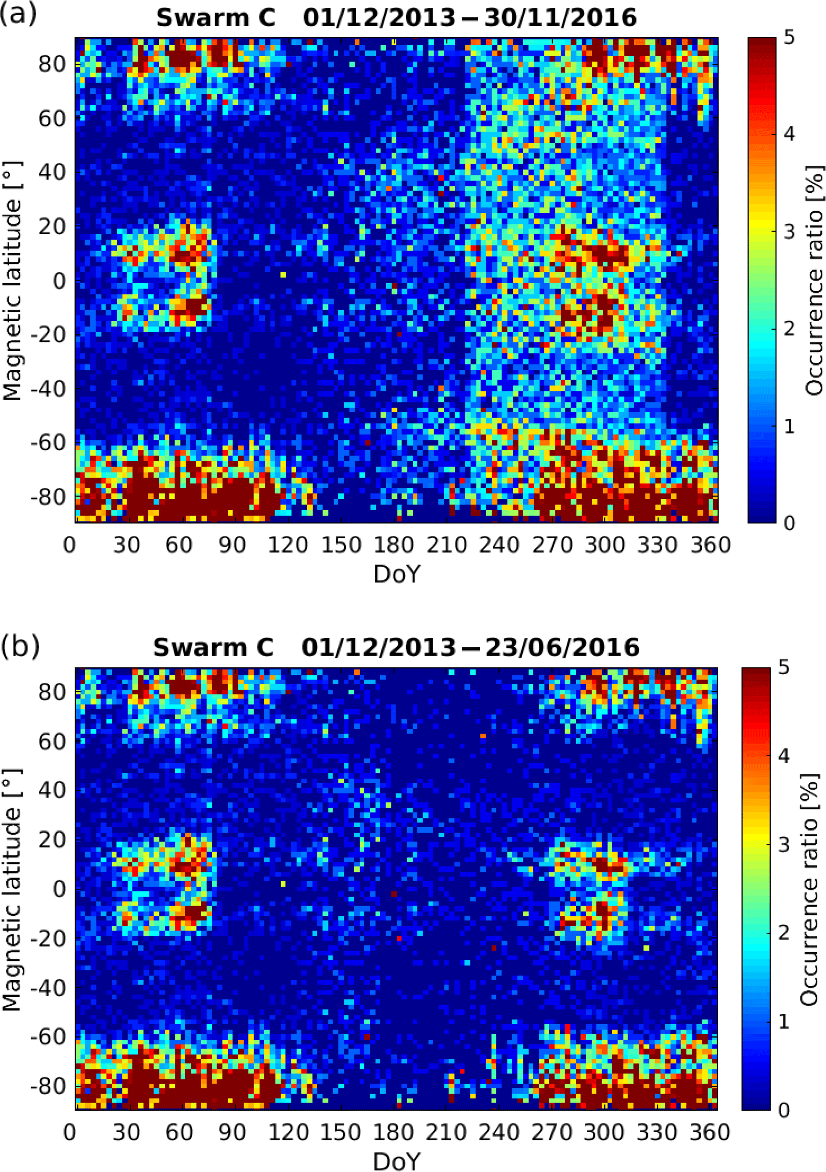
Figure 6The MLAT vs. DoY distribution of the GPS signal loss events observed by Swarm C during (a) 3-year period from 1 December 2013 to 30 November 2016 and (b) from 1 December 2013 to 23 June 2016 before the PLL bandwidth of Swarm C increased to be larger than 0.5 Hz.

Download

3.1 Global and magnetic local time (MLT) dependence of GPS signal loss and the relation to plasma density gradients

Figure 2 presents the global distribution of the GPS signal loss occurrence. For creating the panels of each Swarm satellite, we first sort the events from each GPS satellite into $\mathrm{2}{}^{\circ }\times \mathrm{5}{}^{\circ }$ bins (in geographic latitude and longitude) and then in each bin add up the events from all GPS satellites. Finally, the event numbers are divided by the orbit numbers of Swarm satellite to get the occurrence ratio for each bin. The occurrence of signal loss shows a quite similar global distribution between the three Swarm satellites, with slightly lower values for Swarm B, which flies at about a 50 km higher altitude than the other two. Three latitude bands are highlighted for these events from a global view: one is at low latitudes between ±5 and ±20^∘ magnetic latitude (MLAT), forming two bands along the magnetic equator (white line) and most prominent at longitudes between −135 and 45^∘ E; the other two regions are at high latitudes above 50^∘ $\left|\text{MLAT}\right|$ in both hemispheres, also following the magnetic latitude lines and most prominent at longitudes close to the magnetic poles. Compared to the northern hemisphere, more events are observed in the southern high latitudes, which is similar to the result shown in Fig. 14 of Jäggi et al. (2016) that used 1-month GPS data of Swarm. Additionally, very few events are also observed at middle latitudes around east Asian longitudes.

In Fig. 2, we see the global distributions of signal loss events are quite similar between the three Swarm satellites; therefore, in the rest of this study we show only the observations from the Swarm C satellite. Figure 3a presents the MLAT vs. MLT distribution of GPS signal loss events from Swarm C. The MLT is defined as the solar local time at the magnetic equator and mapped to higher latitudes along the magnetic meridian. For example, MLT =12 (noon) is defining the magnetic meridian facing the Sun at the magnetic equator. Here we used the Quasi-Dipole magnetic field model (Richmond, 1995; Emmert et al., 2010) to calculate MLAT and MLT. Similarly, the events have been first sorted into 2^∘ × 0.5 h bins (in MLAT and MLT, respectively), and then divided by the orbit number of Swarm C in each bin. The low-latitude events appear shortly after sunset (roughly from 19:00 to 23:00 MLT), and are nearly absent during the other hours. This is strong evidence that confirms that the GPS signal loss at low latitude is caused by the post-sunset EPIs, as reported in Xiong et al. (2016a). When looking at high-latitude events, they are observed at almost all local times, but with higher occurrence around noon hours for both hemispheres. Again, it shows higher occurrence at the southern high latitudes. Figure 3b and c show the MLAT vs. MLT distribution in a polar view ($\left|\text{MLAT}\right|\ge \mathrm{50}$^∘). The dayside events show higher occurrence and are located at higher latitude ($\left|\text{MLAT}\right|\ge \mathrm{70}$^∘), and they are possibly collocated with the cusp region (Reiff et al., 1977) in the Southern Hemisphere; while the nightside events prefer to appear at lower latitudes (between $\mathrm{50}{}^{\circ }\le \left|\text{MLAT}\right|\le \mathrm{60}$^∘) and are possibly collocated with the auroral oval (Feldstein, 1963; Akasofu, 1966) in both hemispheres. Scintillations on the radio wave signals have already been reported at high latitudes (e.g., Martin and Aarons, 1977; Rino et al., 1978; Aarons et al., 1997), and evidence showed that they are highly related to these high-latitude irregularities (e.g., Meeren et al., 2015; Oksavik et al., 2015; Jin et al., 2015; Clausen et al., 2016). The GPS signal loss of Swarm satellites at high latitudes is also believed to be caused by the irregularities. These high-latitude plasma irregularities, including polar cap patches occurring inside the polar cap (Crowley, 1996; Clausen and Moen, 2015) and auroral blobs at aurora latitudes (Crowley et al., 2000; Jin et al., 2014), can be created directly/indirectly by particle precipitations (Kelley et al., 1982) or through the convection of dayside plasma into the polar cap (Foster et al., 2005; Stolle et al., 2006b).

To check if the high-latitude GPS signal loss also depends on the amplitude of plasma gradients, we further analyzed Swarm in situ plasma density measurements. Figure 4a shows such an example at high latitudes. The original 2 Hz electron density data measured by the Langmuir probe is plotted with a black line, and a filter has been applied to the original data series for filtering out irregularities with scale lengths of less than 120 km along track, following the work of Xiong et al. (2016b). From the filtered data (red line) we then find all depleted regions, and the peak values between two depleted regions are then recorded from the original 2 Hz data series (marked with green squares). Then the minima between two peak values are found (also from the original data series and marked with blue triangles). For each depleted region, the density gradient (ΔNe) is then defined as the larger value between the minima (blue triangles) and two neighboring peaks (green squares). The two pink crosses indicate where the largest gradient Δ Ne_max are found during this orbital arc. In this way, we derived the along-track plasma density gradients from each Swarm high-latitude pass (orbit arc with $\left|\text{MLAT}\right|\ge \mathrm{50}$^∘).

Figures 4b and 4c present the MLAT vs. MLT distribution of the density gradient for the northern and southern hemispheres, respectively, and only the passes with GPS signal loss observed have been taken into account. The density gradient generally show larger values at 70–80^∘ $\left|\text{MLAT}\right|$ on the dayside (09:00–15:00 MLT) and at 60–70^∘ $\left|\text{MLAT}\right|$ on the nightside. This kind of distribution, with largest plasma density gradients in the cusp region at noon and with a “tail” reaching from afternoon to midnight at lower latitudes at 60–70^∘ $\left|\text{MLAT}\right|$, is considered to be caused by the tongue of ionization (TOI) phenomenon, which is attributed to be a major source of polar patches (e.g., Hosokawa et al., 2010; Carlson, 2012). Figures 4d and e present the electron density gradient distribution derived only from the orbits without GPS signal loss events detected. Although the structure of TOI can also be seen here, the density gradient amplitudes have been reduced by a factor of 2 (or even larger) compared to Fig. 4b and c, which also confirms that the density gradients with larger amplitude is an essential factor for causing GPS signal loss of Swarm satellites.

To better quantify the relation between high-latitude plasma gradients and GPS signal loss events, Fig. 5a presents the MLT distribution of ΔNe_max. For each high-latitude pass, we take only the maximum density gradient (ΔNe_max, the difference between the two pink crosses as shown in Fig. 4a), and considered the GPS signal loss within ±3 min where the ΔNe_max is observed. The black dots represent the ΔNe_max without GPS signal loss observed and the other ΔNe_max are marked with different colors when signal loss happened at different PRN numbers. It obviously shows that the signal loss at more channels prefers to happen when Swarm encountered larger density gradients. If we consider orbital arcs with only ΔNe${}_{\text{max}}\ge \mathrm{5}\times {\mathrm{10}}^{\mathrm{11}}$ m⁻³ (Fig. 5b), the chances of GPS signal loss happened at least for one channel, with tracked GPS satellites less than 4 (precise orbit determination is impossible), and the chances of a signal loss at all eight channels are 94.3, 9.4, and 0.5 %, respectively. For orbital arcs with ΔNe_max between 2.5×10¹¹ and 5×10¹¹ m⁻³ (Fig. 5c) and between 1×10¹¹ and 2.5×10¹¹ m⁻³ (Fig. 5d), the chances for the three situations are reduced to 77.8, 2.1, and 0.1 and 28.5, 0.8, and 0.0 %, respectively. When only considering orbital arcs with very low-density gradients (ΔNe${}_{\text{max}}<\mathrm{1}\times {\mathrm{10}}^{\mathrm{11}}$ m⁻³, Fig. 5e), nearly no GPS signal loss events are observed. The result quantitatively confirms that only those plasma gradients (associated with high-latitude plasma irregularities) with absolute amplitudes large enough can cause the GPS signal loss, which is also consistent with that at low latitudes as shown in Fig. 8 of Xiong et al. (2016a).

3.2 Seasonal dependence of GPS signal loss

We further checked the seasonal dependence of GPS signal loss events. The events are first sorted into 2^∘ MLAT and 3 day (by day of year, DoY) bins, and then divided by the total orbit number of Swarm C in each bin to get the occurrence ratio. As shown in Fig. 6a, a clear seasonal pattern is found at both low and high latitudes, that the signal loss has higher occurrence during equinoxes and December solstice months, while relatively low during June solstice months. Additionally, unexpected occurrences are found at all latitudes during DoY from 224 (11 August) to 335 (30 November). We checked the updates to the Swarm receiver and found that the PLL bandwidth of Swarm C had been increased from 0.75 to 1.0 Hz on 11 August 2016 (see Table 1), and the unexpected signal loss events are possibly observed after this update. When we considered the dataset before PLL bandwidth increased to 0.75 Hz (until 11 August 2016) or even earlier until 23 June 2016 (PLL bandwidth still at 0.5 Hz), the unexpected signal loss events observed at all latitudes from 11 August to 30 November disappeared, and the events observed from 23 June to 11 August mainly at middle latitudes also reduced (Fig. 6b). The comparison in Fig. 6 suggests that some unexpected GPS signal loss events (not related to the ionospheric irregularities) appear just after the PLL bandwidth has increased larger than 0.5 Hz. Further discussion will be given in Sect. 3.4 about the influence of the PLL bandwidth increase on the receivers.

As the GPS signal loss at low latitudes is caused by the EPIs, similar seasonal dependences are expected from them, e.g., higher occurrence around equinoxes and December solstice months from a global view (Burke et al., 2004; Su et al., 2006; Stolle et al., 2008; Xiong et al., 2010). However, the seasonal dependence of polar patches is still an open issue: some studies reported that the polar patches are mainly a local winter phenomenon in both hemispheres (e.g., Coley and Heelis, 1998; Kivanç and Heelis, 1998; Carlson, 2012; Spicher et al., 2017), while there are also studies found that polar patches have higher occurrence during December solstice months in both hemispheres (e.g., Noja et al., 2013; Chartier et al., 2018). Our result shown in Fig. 6 reveals that in both hemispheres the GPS signal losses have a higher occurrence during December solstice, supporting the conclusion of Noja et al. (2013) and Chartier et al. (2018) that the polar patches have higher occurrence at this season. The possible reason for explaining the different seasonal dependence of polar patches is that Spicher et al. (2017) used a method with relative threshold for identifying polar patches (the enhancement must be at least twice that of the background density), while the detection approach used by Noja et al. (2013) was based on a mixture of absolute and relative patch magnitudes (besides the relative enhancement, the absolute TEC enhancement must be larger than 4 TECU; 1 TECU =10¹⁶ electrons m⁻²). Noja et al. (2013) pointed out that the TEC in the Southern Hemisphere exhibited very small magnitudes rarely exceeding 5 TECU during June solstice, hence their detection algorithm possibly ignore most of the patches, but these small magnitude patches will possibly be detected by Spicher et al. (2017) when they only concern the relative enhancements. A detailed discussion about the difference between Noja et al. (2013) and Spicher et al. (2017) has also been provided in Charter et al. (2018). Our result reveals that for causing the receiver connection loss with GPS satellites, the plasma density gradients along the signal path must exceed a certain threshold.

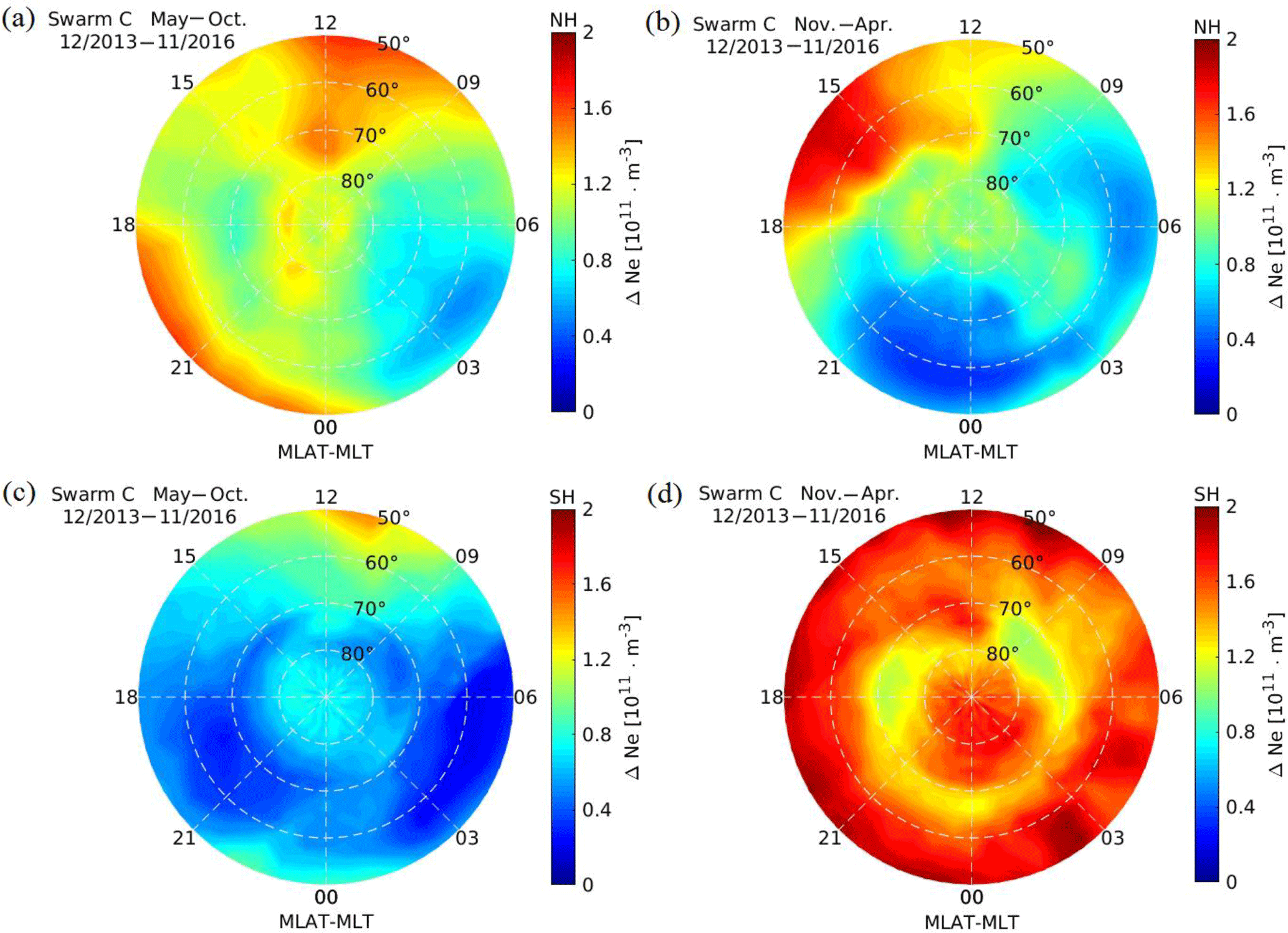
Figure 7The MLAT vs. MLT distribution of the ionospheric background density in the (a, b) northern and (c, d) southern hemispheres during two periods: (a) and (c) from May to October when almost no signal loss events were observed and (b) and (d) from November to April when most of the signal loss events were observed.

Download

We further checked the ionospheric background density measured by the Swarm C for the two different periods: November–April (when most of the GPS signal losses are observed) and May–October (nearly no GPS signal loss observed). For the northern high latitudes, the background plasma density during May–October (local summer, Fig. 7a) is slightly larger than that during November–April (local winter, Fig. 7b). However, for the Southern Hemisphere, the background plasma density is very low during local winter (Fig. 7c) and large during local summer (Fig. 7d). It is known that at high latitudes, the solar radiation during local summer is larger than that during local winter, and from a global view the F-region ionospheric plasma density is larger during December solstice than during June solstice, which is also well-known as the F-region annual anomaly (Torr et al., 1980; Rishbeth and Müller-Wodarg, 2006). The two effects are balanced in the Northern Hemisphere, that's why we see smaller summer–winter asymmetry of the background plasma density in the Northern Hemisphere; while the two effects are adding together in the Southern Hemisphere, causing larger summer–winter asymmetry of the ionospheric background density in the Southern Hemisphere. The result shown in our Fig. 7 also indicates that the polar patches during the southern winter, although with high occurrence (Spicher et al., 2017), are associated with very low-density gradients that will hardly cause GPS signal loss of the receivers, but those patches during southern local summer associated with high-density gradients have the potential to disturb the GPS signals.

3.3 Orientation dependence of GPS signal loss

The low-latitude irregularities derived from TEC measurements show a typical orientation dependence, which is strongest when the corresponding GNSS satellite is westward of the receiver with elevation angles of about 40–60^∘ (Park et al., 2015), and TEC gradients at high latitudes are also found to be strongest when the line of sight (LOS) between the receiver and GNSS satellites is most aligned with the ionospheric L-shell surface (Park et al., 2017). Therefore, we also checked if a similar orientation dependence can be found for the Swarm GPS signal loss events.

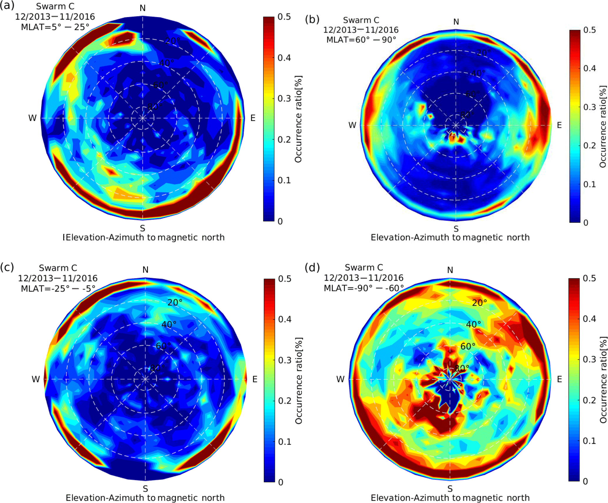
Figure 8The elevation and azimuth distribution of GPS signal loss events at (a) northern and (c) southern low latitudes observed by Swarm C. The azimuth angle is calculated with respect to the magnetic north. (b) and (d) are similar to (a) and (c) but for the high latitudes in both hemispheres.

Download

Figure 8 presents the elevation and azimuth distribution of GPS signal loss occurrence. The elevation angle of 0^∘ (90^∘) means the GPS satellite is just horizontal (overhead) compared to Swarm, and the azimuth angle of 0^∘, 90^∘, 180^∘, and 270^∘ means the GPS satellite is at the north, east, south, and west compared to the Swarm satellite, respectively. As the ionospheric structures, e.g., EPIs and polar patches, prefer to follow magnetic coordinates rather than geographic coordinates, here we show the results with azimuth angles calculated to the magnetic north. The events from all GPS satellites are sorted into $\mathrm{5}{}^{\circ }\times \mathrm{10}{}^{\circ }$ bins (in elevation and azimuth, respectively) and divided by the observed GPS satellite numbers (in total) to get the occurrence ratio for each bin. Results are shown separately for low (panels a and c) and high latitudes (panels b and d) in both hemispheres. At low latitude, we considered events within 5 to 25^∘ and −25 to −5^∘ MLAT for representing the northern and southern EIA crest regions, respectively. Most of the signal loss events are observed with elevation angles of less than 20^∘ in both hemispheres, and four outstanding regions are found with azimuth angles around 45^∘ (northeast), 135^∘ (southeast), 225^∘ (southwest), and 315^∘ (northwest), while minimum activities are found for east and west LOS directions. This orientation dependence is possibly related to the shell structure of EPIs. For EPIs with westward-tilted (“inverted-C” shell structure, proposed by Kil et al., 2009), the LOS directions of GPS satellites from southwest and northwest direction are mostly aligned with the EPIs extension with respect to the Swarm receiver, causing the signal loss events highlighted at orientation with azimuth angle around 225 and 315^∘. However, as pointed out by Huba et al. (2009), the shell structure of EPIs can be tilted with different angles, depending on the background zonal wind. If EPIs are eastward-tilted (“C” shell structure), the LOS direction of GPS satellites from the northeast and southeast directions are then mostly aligned with the EPIs extension, as a result we see the signal loss events also highlighted at orientation with azimuth angle around 225 and 315^∘, respectively. As shown in Wu et al. (2017), EPIs usually have a larger north–south extension (about 1000 km) than the east–west extension (about 50 km), which also means EPIs are largely aligned with the magnetic north–south direction. That is, for low elevation angles close to the horizon (e.g., <20^∘) east–west LOS directions are nearly normal to EPI surfaces while north–south LOS directions are nearly tangent to the surfaces. Hence, the former LOS directions lead to a negligible or weak along-track gradient of slant TEC because a part of the LOS should always be affected by the EPI shell. The east–west LOS directions cannot result in significant degradation of GPS signal quality. This explains the general lack of signal loss events in the east–west LOS directions as shown in Fig. 8a and c.

Another interesting feature seen here is that when Swarm C is at the northern crest region, some signal loss events with elevation angles larger than 20^∘ are found from the GPS satellites toward the south (azimuth angle around 180^∘), but almost absent from the GPS satellites toward the north (azimuth angel around 0^∘). This can be explained as when the Swarm satellite is in the northern crest region, no plasma irregularities exist in the northern middle latitudes, but the EPIs from the Southern Hemisphere still affects the GPS signal when the LOS direction of signal propagation is aligned with EPIs extension. A mirrored distribution is found when Swarm C is at the southern crest region, and the same explanation applies here.

Figure 8b and d present the GPS signal loss events at high latitudes ($\mathrm{60}{}^{\circ }\le \left|\text{MLAT}\right|\le \mathrm{90}$^∘) as a function of elevation and magnetic azimuth angles. In the Northern Hemisphere, most of the events are still with elevation angles less than 20^∘, but events with elevation angles up to 50^∘ are also observed. The anisotropy is also related to the morphology of high-latitude ionospheric irregularities. For a low-elevation angle (e.g., <20^∘) at high-latitude regions, the east–west direction is nearly tangent to the local L-shell while the north–south direction is perpendicular to it. Because the high-latitude irregularities are generally aligned with local L-shells (Park et al., 2017), Swarm should experience a stronger along-track gradient of slant TEC for east–west LOS directions (i.e., LOS directions tangent to the irregularity surface) than for north–south LOS directions (i.e., LOS directions perpendicular to the irregularity surface). Note that for the latter case, a part of LOS is always immersed inside the irregularity, which leads to negligible along-track gradient of slant TEC. The weak along-track gradient cannot significantly degrade GPS signal quality. On the other hand, in the Southern Hemisphere the events are extended to almost all directions. Due to a larger offset between geographic and magnetic poles and related insolation effects in the Southern Hemisphere, ionospheric irregularities are not well aligned with local L-shells (Park et al., 2017). Hence, it is expected that the preference for east–west LOS directions is conspicuous in the Northern Hemisphere and weak in the Southern Hemisphere.

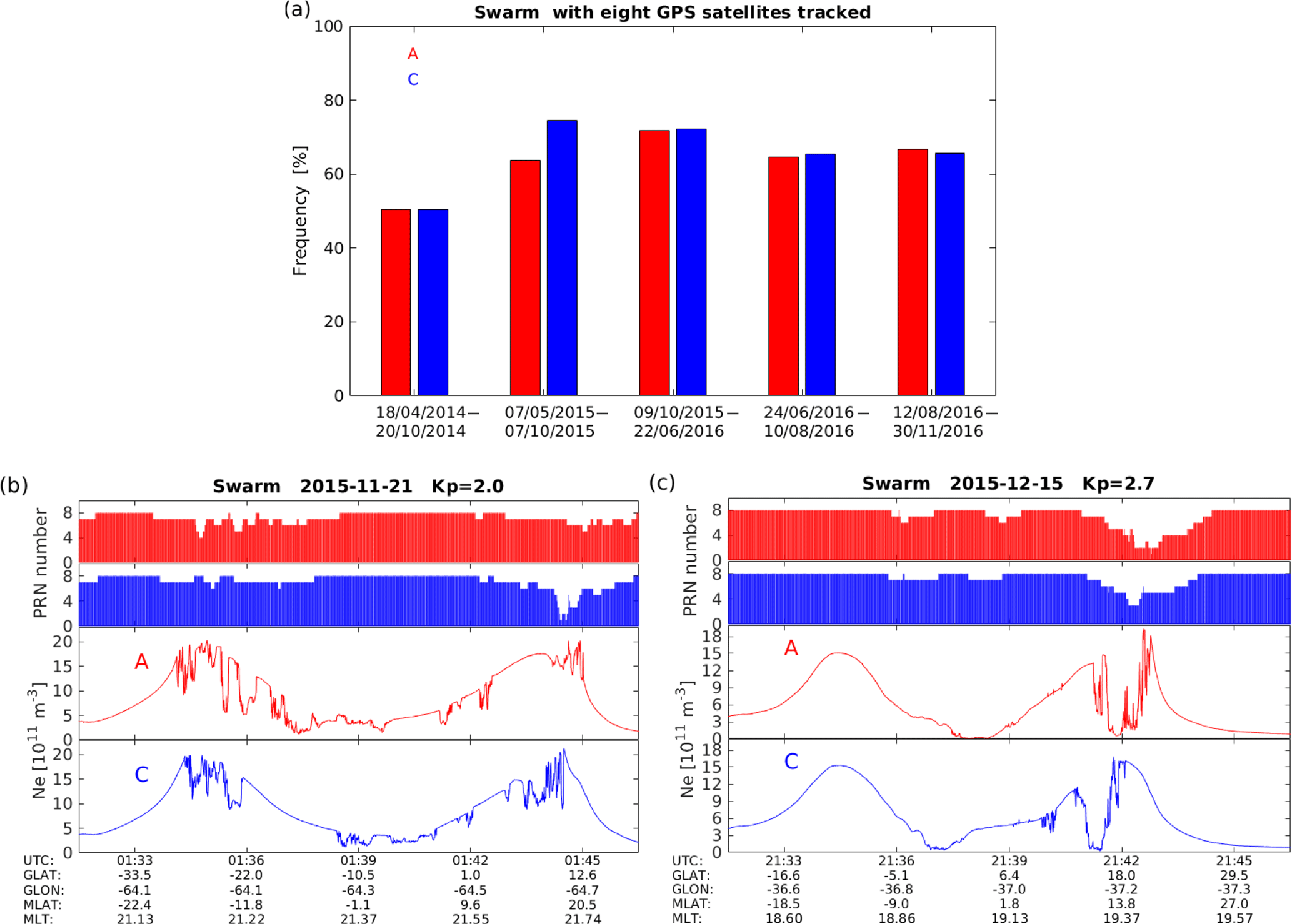
Figure 9(a) The occurrence of tracked GPS satellites at all eight channels for Swarm A (red) and C (blue) during five different periods: (1) from 18 April 2014 to 20 October 2014 when the FOV and PLL bandwidth have not been updated for both satellites; (2) from 7 May 2015 to 7 October 2015 when the FOV of both Swarm A and C have increased from 80 to 88^∘, while the PLL bandwidth is 0.25 and 0.5 Hz for Swarm A and C; (3) from 9 October 2015 to 22 June 2016 when the PLL bandwidth is both 0.5 Hz for Swarm A and C; (4) from 24 June 2016 to 10 August 2016 when the PLL bandwidth is 0.5 and 0.75 Hz for Swarm A and C; and (5) from 12 August 2016 to 30 November 2016 when the PLL bandwidth is 0.75 and 1.0 Hz for Swarm A and C. (b) and (c) are two examples of equatorial plasma irregularities observed by Swarm A and C during the third period when both the FOV and PLL bandwidth have been updated. However, the GPS receivers onboard both satellites were still found with signal loss at some channels during both events.

Download

3.4 Performance of GPS receiver before and after PLL bandwidth increase

As introduced in Sect. 2.1, the FOV and PLL bandwidth of the Swarm GPS receiver have been updated several times during the Swarm mission. The increased FOV definitely helps the Swarm receivers to keep track with GPS satellites of low elevation angles, but it provides less help when Swarm satellites encounter plasma irregularities with large gradients. The PLL bandwidth has also been widened, in attempt to increase the robustness against scintillation. However, as discussed in Fig. 6, after the PLL bandwidth of Swarm C has gradually increased from 0.5 to 1.0 Hz, some unexpected GPS signal loss events (not related to plasma irregularities) were observed even at middle latitudes. Since Swarm A and C are flying side by side with a longitudinal separation of only 150 km at low and middle latitudes, their receivers are expected to undergo similar condition for receiving GPS signals. However, their PLL bandwidth were updated on different dates, therefore, taking the occurrence of tracked GPS satellites at all eight channels as an example, we have compared the two receivers' performance during periods of different bandwidth.

As shown in Fig. 9a, five periods have been taken into account. The first period is from 18 April to 20 October 2014, both PLL bandwidth and FOV have not been updated for Swarm A and C, and we see that during 50.5 and 50.3 % of the time Swarm A and C, respectively, can track eight GPS satellites. For the second period from 7 May 2015 to 7 October 2015, the FOV of both Swarm A and C had increased from 80 to 88^∘, and the PLL bandwidth of only Swarm C has been increased from 0.25 to 0.5 Hz, while it stays at eight 0.25 Hz for Swarm A. Then we see the occurrence of tracking of eight GPS satellites has been increased to 74.6 % for Swarm C, which is 10.8 % higher than Swarm A. During the third period from 9 October 2015 to 22 June 2016, the PLL bandwidth are both at 0.5 Hz for Swarm A and C, and the percentage with eight GPS satellite tracked increases to 71.7 and 72.1 % for the two satellites. However, the increase of about 20 % for reception at all eight-channels between the first and third period cannot solely be attributed to the increased bandwidth, but also partly expected to be caused by the decreasing solar flux (F10.7) from about 145 sfu (unit of solar flux index, f10.7, sfu=10⁻²²W m⁻² Hz⁻¹) in the middle of 2014 to about 90 sfu in June of 2016, resulting in a lower background plasma density. For the remaining two periods, although the PLL bandwidth increased again for Swarm A and C and the solar activity stays at a low level, the occurrence of tracking of eight GPS satellites are somehow slightly reduced (by about 5 %) for both of them. No doubt that the increased PLL bandwidth can improve the capability of the receiver to keep track with GPS signal, but if the bandwidth has been widened too much, the noise level of the GPS signal will also increase; and as a result (see Fig. 6) the receiver will suffer a side effect and will be more easily disturbed. Our results suggests that rather than 1.0 Hz, a PLL bandwidth of 0.5 Hz is a more suitable value for the Swarm receiver.

Additionally, events with GPS signal losses at several channels are still observed after the PLL bandwidth increased. Two such examples are presented in Figs. 9b and c. During the first event on 21 November 2015 when the PLL bandwidth of Swarm A and C have been increased to 0.5 Hz, the number of tracked GPS satellites reduced from 8 to 4 (at the southern EIA crest), and from 8 to 1 (at the northern EIA crest) for Swarm A and C, respectively; during the second event on 15 December 2015, the number of tracked GPS satellites for Swarm A and C at both the northern EIA crest reduced to 2 and 3, respectively. These are encouraging results to further investigate the GPS signal loss for onboard receivers with selected settings.