the Creative Commons Attribution 4.0 License.
the Creative Commons Attribution 4.0 License.
 | 16 Apr 2018
A critical note on the IAGA-endorsed Polar Cap (PC) indices: excessive excursions in the real-time index values
The Polar Cap (PC) indices were approved by the International Association for Geomagnetism and Aeronomy (IAGA) in 2013 and made available at the web portal http://pcindex.org holding prompt (real-time) as well as archival index values. The present note provides the first reported examination of the validity of the IAGA-endorsed method to generate real-time PC index values. It is demonstrated that features of the derivation procedure defined by Janzhura and Troshichev (2011) may cause considerable excursions in the real-time PC index values compared to the final index values. In examples based on occasional downloads of index values, the differences between real-time and final values of PC indices were found to exceed 3 mV m−1, which is a magnitude level that may indicate (or hide) strong magnetic storm activity.
Keywords. Magnetospheric physics (solar wind–magnetosphere interactions; polar cap phenomena) – ionosphere (modelling and forecasting)
- Article
(4389 KB) -
Supplement
(6534 KB) - BibTeX
- EndNote


The Polar Cap (PC) indices, PCN (North) based on magnetic data from Qaanaaq (Thule) and PCS (South) based on Vostok data, reflect the transpolar convection of plasma and magnetic fields. They have important applications for space weather analyses and forecasting and have been used in many publications (e.g. Stauning, 2013a, and references therein). The PC indices could be used, among others, to indicate the energy transfer from the solar wind to the magnetosphere–ionosphere–thermosphere system (e.g. Troshichev et al., 2014).
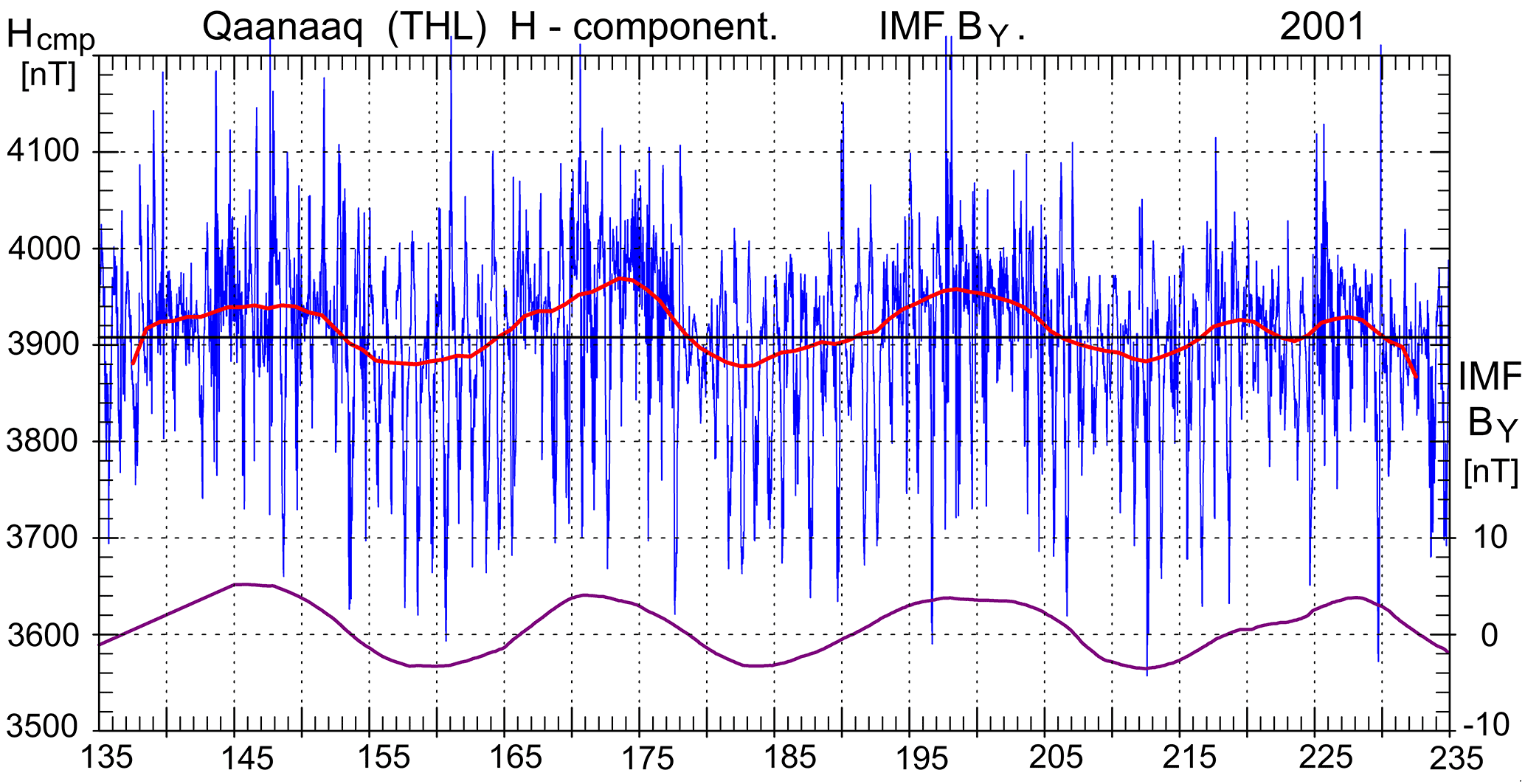
Figure 1H-component data (20 min avg.) from Qaanaaq for days 135–235 of year 2001 in the blue line. Smoothed H-component median values in the red line. Smoothed IMF BY values in the magenta line on the right scale.
PC index values are calculated from the basic formula (e.g. Troshichev et al., 2006) by
where ΔFPROJ is the horizontal polar magnetic variation vector ( counted from a reference quiet level (FQL) and projected to a specific optimum direction in space considered to be perpendicular to the transpolar forward (noon to midnight) plasma convection direction. The optimum direction is defined through its angle, φ, with the E–W meridian, while the slope, α, and the intercept, β, are calibration parameters. The parameters (φ, α, and β) are tabulated for each minute through the year (e.g. http://pcindex.org). They are invariant over years.
The PC indices in the formulation suggested by the suppliers, the Arctic and Antarctic Research Institute (AARI) in St. Petersburg, Russia, and DTU Space in Lyngby, Denmark, were approved by the International Association for Geomagnetism and Aeronomy (IAGA) by Resolution no. 3, 2013 (http://www.iaga-aiga.org/resolutions). In the resolution “IAGA … recommends use of the PC index by the international scientific community in its near-real time and definitive forms”. The IAGA approval was given on the basis of documentation summarized in Appendix A (2014) referring to the publications Troshichev et al. (2006), Janzhura and Troshichev (2008, 2011), and Troshichev and Janzhura (2012). Index values derived by the IAGA-approved method are distributed from the PC index web site http://pcindex.org and from the web portal http://isgi.unistra.fr/data_download.php of the International Service of Geomagnetic Indices (ISGI). A description of the PC indices and their derivation is provided in Troshichev (2011).
An essential element of the calculation of PC index values is the derivation of the quiet reference level (QL), from which the disturbance amplitudes are counted. The QL derivation method described in Janzhura and Troshichev (2011, hereafter J&T2011) used for calculation of archival (final) index values was discussed in Stauning (2013b, 2015). This method uses data recorded approximately one month before and after the day in question to derive the relevant daily varying quiet level.
For calculation of real-time PC index values, the scaling parameters (φ, α, and β) are those used for the final index values. A special procedure was developed to derive the actual QL from past (pre-event) magnetic data only (J&T2011). As post-event data become available, the procedure includes the added data to recalculate QL and PC index values, which are gradually turned into archival values. The available documentation is rather sparse in the description of the procedure and does not provide examples of real-time QL or PC index values. The real-time procedure and examples from occasional downloads of actual PC index values are discussed here in order to identify and quantify the problems with the IAGA-endorsed methodology.
The transitions between the various states of processing of PC index values are not defined in the documentation supplied for the IAGA endorsement. Here, the designation “archival” (or “final”) values shall be used on PC indices retrieved one or more years after the index date assuming that the magnetic data of importance and their processing have been finalized. The term “prompt” values shall be used for downloads of one month's worth of PC indices up to and including the actual “real-time” values. Within this interval, the database for QL derivation is definitely changing. PC indices from the two days of current data on display at http://pcindex.org are termed “near-real-time” values. These definitions shall be maintained in posterior data processing attempting to emulate downloads of prompt PC indices.
The quiet reference level for the horizontal magnetic field vector, FQL, (HQL, DQL) or (XQL, YQL), could be considered built from the secularly varying base level, FBL, adding the daily variation, FQDC, observed during quiet days (quiet day curve, QDC).
For illustration, Fig. 1 presents the H component of magnetic data (blue line) measured at Qaanaaq (Thule). The interval of data, days 135–235 of year 2001, is much the same as that used in Fig. 1 of J&T2011. The base level, HBL, is marked by the solid horizontal line. The excursions from the base level relate to the combination of quiet day variations to be omitted and magnetic disturbances to be included at PC index calculations. The varying transverse component, IMF BY, of the interplanetary magnetic field (IMF) displayed in a smoothed version (the magenta line) at the bottom of Fig. 1 appears to impose systematic variations on the recorded level.
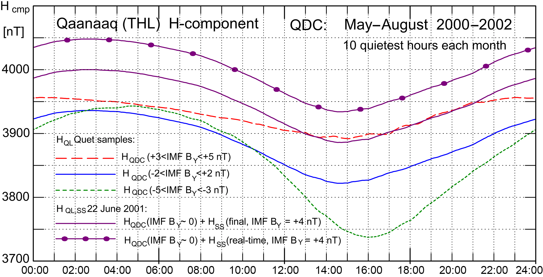
Figure 2Qaanaaq (Thule) H-component data averaged through the 10 quietest hours of the summer months in 2000–2002 for groups of data with −5 < IMF BY < −3 nT (green dotted line), −2 < IMF BY < +2 nT (solid blue line), and +3 < IMF BY < +5 nT (red dashed line), respectively. HQL,SS for 22 June 2001 in “final” (solid magenta line) and “real-time” (magenta line with dots) versions (see text). Local solar and magnetic noon are at around 16 UT.
The H-component daily median values have been Gaussian smoothed through 7 days (e-folding period = 2 days). The resulting median values presented by the wavy curve (the red line) in Fig. 1 are modulated much like the smoothed IMF BY values, which have a dominant period at or close to the 27 days solar rotation period. The systematic modulation of the IMF BY patterns relates to shifts between sustained away and toward solar magnetic field directions within solar wind sectors (e.g. Svalgaard, 1973). The effects on the magnetic data are caused by IMF BY-related changes in the polar plasma convection patterns particularly close to the dayside cusp region located near noon in magnetic local time (MLT). The IMF BY-related effects are enhanced by high ionospheric conductivities at local time (LT) noon, in the summer season, and at solar maximum (e.g. Friis-Christensen et al., 1985).
Figure 1 conveys the impression that the recorded H-component level varies systematically, both day and night, by a slowly varying amount related to IMF BY. In an attempt to compensate for such level changes, Troshichev (2011) introduced a solar wind sector (SS) term, which for each component of the recorded magnetic field is the difference between the long term average (horizontal line in Fig. 1) and the daily median value with adequate smoothing (superimposed wavy curve in Fig. 1). For the resulting reference QL, it is stated in J&T2011 (p. 1499) that “this level of reference can be derived if the SS effect is taken into account prior to the QDC derivation”.
A comprehensive description of the derivation of the QL reference level, from which the disturbances are counted, is not available. The computer program description (function pc_db in Appendix A, 2014) in the PC index documentation supplied to IAGA shows that the solar wind sector term is added as a specific contribution to the quiet level as well as taken into account in the QDC derivation. Thus, in the IAGA-endorsed version, the quiet reference level, FQL,SS, could be considered built from the secularly varying base level, FBL, the quiet daily variation, FQDC,SS, and a solar wind sector term, FSS, according to Eq. (2):
The IAGA-endorsed QDC procedure (function qday_db in Appendix A, 2014) is described in Janzhura and Troshichev (2008, hereafter J&T2008). An initial QDC for each component is calculated by superposition of samples of quiet data collected through an interval of 30 days to determine the daily variation for one day at a time. Depending on the distribution of quiet samples, this day is usually positioned at the middle of the interval. A series of initial QDCs is calculated by shifting the 30-day period by 10 days at a time. The final QDCs for all days are now found by smoothing interpolation through the series of initial QDCs
To provide an illustration of the quiet daily variation, Fig. 2 presents QDCs made from hourly averages of the H component of the magnetic field measured at Qaanaaq during the 10 quietest hours of each month of the summer periods (May–August) of 2000–2002. The data are grouped according to the IMF BY level. Data for the interval −5 < IMF BY < −3 nT are represented by the green dotted curve, −2 < IMF BY < +2 nT by the solid blue curve, and +3 < IMF BY < +5 nT by the dashed red curve.

Figure 3(a) Calculation of HSS from 3-day median values (green curve), based on data available up to and including 13 June (from Fig. 6b of J&T2011), using cubic spline interpolation (black line) on 3-day medians between 6 and 12 June (dots on green curve) and extrapolation to define HSS=91 nT on 14 June (large black dot). Resulting HSS values for June (so far) are displaced 60 nT downward and connected by a dashed line using the lower right scale. (b) cubic spline interpolation on 3-day median samples between 9 and 15 June to define HSS=21 nT on 17 June. (c) cubic spline interpolation on samples between 14 and 20 June to define HSS=112 nT on 22 June. (d) Cubic spline interpolation between 19 and 25 June to define nT on 27 June. Smoothed IMF BY values are displayed at the top of the diagrams using the upper right scale.
These three curves in Fig. 2 represent the expected daily variation, HQDC, with sustained IMF BY levels within the defined limits and for the epoch considered. Local (LT and MLT) noon at Qaanaaq is at around 16 UT. The night HQDC values (00–08 UT) are not changed much with differing IMF BY, while the daytime HQDC values (12–20 UT), and thus the amplitude in the daily variation, change considerably with the varying IMF BY level. For the three cases, the IMF BZ conditions are about the same with average values ranging between −0.1 and +0.1 nT.
For the J&T2008 QDC procedure, the contributions from the IMF BY-related positive and negative level shifts over the 30-day interval considered at a time tend to balance each other (cf. Fig. 1). For the examined interval, days 135–235 of 2001, as an example, the average IMF BY over any 30-day subsections range between −0.7 and 1.2 nT. Thus, the quiet daily variation for the SS-corrected data, HQDC,SS, is most likely close to the result obtained for the case −2 < IMF BY < +2 nT (the solid blue curve in Fig. 2). Consequently, the sector effect on the QL is mainly provided by the addition of the slowly varying term, HSS, (cf. Eq. 2) to the daily course found at IMF BY≈0. The addition will change the daytime and the nighttime parts of the QLs by similar amounts without changing the amplitude in the daily variation.
This is illustrated in Fig. 2 by the solid magenta curve where, as an example, the HSS term (64 nT) in the final version from J&T2011 for day 173 (22 June) of 2001 has been added to the HQDC for IMF BY≈0 (blue solid line) to provide the HQL,SS variations for the day according to Eq. (2). On this day, IMF BY (smoothed) ≈4 nT (see Fig. 1). The expected QL based on quiet samples only is represented by the HQDC curve for 3 < IMF BY < 5 nT (red dashed curve) in Fig. 2. It is seen that the HQL,SS resulting from Eq. (2) matches the expected HQDC level at daytime, while large differences appear at night causing PC index changes that may not be justified by the actual magnetic variations. In order to ease comparisons of real-time and post-event QL methods, the curve marked by dots (in magenta) in Fig. 2 displays the HQL,SS variations on 22 June obtained by addition of the real-time HSS=112 nT for this day (cf. Fig. 3c) to the HQDC for IMF BY≈0.
The QL derivation for archival (post-event) data in the IAGA-endorsed procedure is discussed in Stauning (2013b, 2015). The main problem for the procedure is the incorrect assumption that the IMF BY-related level changes are the same day and night. As seen in Fig. 2 for the quiet samples, in Fig. 5 of J&T2011 for all data samples, or by separate displays of the daytime and nighttime data (Stauning, 2015), the IMF BY-related effects on the H components are strong during daytime only. The addition of the same term, HSS, to daytime as well as nighttime QLs causes the nighttime reference levels to step up or down with IMF BY instead of remaining steady. The problem is aggravated by the still larger HSS amplitudes found by using the real-time QL version.
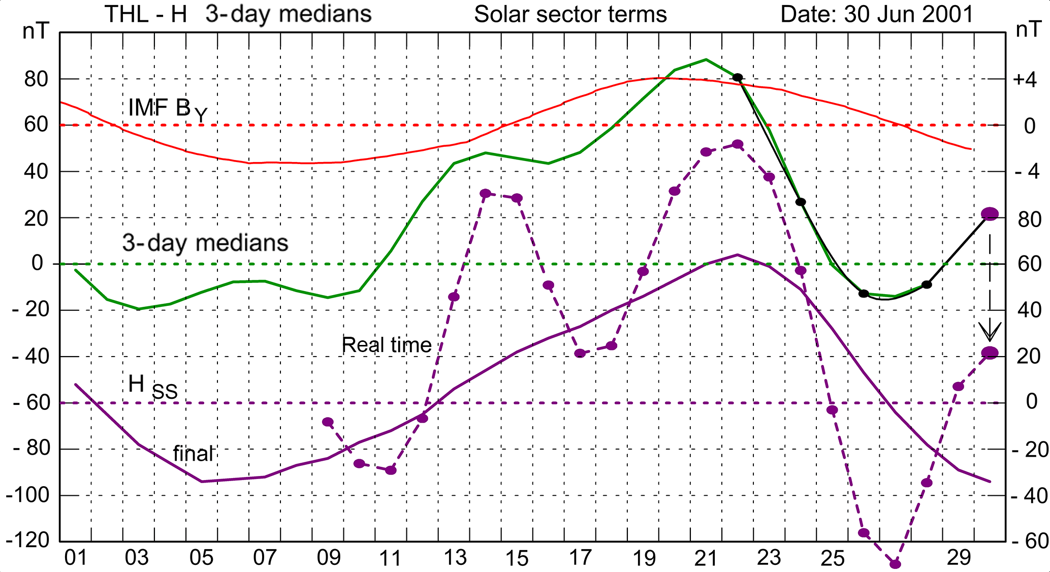
Figure 4Calculation of HSS=21 nT for 30 June from 3-day medians from 22, 24, 26, and 28 June. The 3-day median values (from Fig. 6b of J&T2011) are shown in green line. The HSS values from Fig. 6b of J&T2011 are shown by the smooth solid magenta line on the scale to the right, while the HSS values calculated here by cubic spline extrapolation are shown on the same scale by dots connected by the dashed magenta line.
The derivation of the reference QL in real time poses further challenges. As indicated in Eq. (2), the QL (IAGA-endorsed version) comprises a QDC and an additional solar wind sector (SS) term. The QDC procedures described in J&T2008 comprise a real-time option, where the most recent completed QDCs are projected forward in time by using the seasonal trend obtained from stored QDCs derived at corresponding times in past year(s). It is not clear how to derive the proper trend if past QDCs are based on data corrected for the SS effects, which could not be taken to repeat a year later. This issue, left unresolved, is considered a minor problem compared to the derivation of the SS term in real time.
The J&T2011 publication describes the SS-related contribution to the reference quiet level (cf. Eq. 2), from which the magnetic variations used in the derivation of PC index values are counted. The SS term relies on median values of the recorded data. The daily medians display large fluctuations from day to day. In the post-event processing, these fluctuations are reduced according to J&T2011 by smoothing the daily medians over 7 days centred at the day in question. Such smoothing is not possible at real time applications where, in addition to missing the median value for the present day (which may not have ended), median values for 3 future days are lacking. The procedure for deriving the real-time SS terms, as defined in J&T2011 (1496–1497), is quoted below.
“Keeping in mind this specification, the 3-day smoothing averages of the median values were subjected to the interpolation procedure including the following steps:
median values for magnetic components H and D are derived for 4 intervals of preceding days with the exception of the current day (n=0):
r1=F[for interval from n−3 day to n−1 day]
r2=F[for interval from n−5 day to n−3 day]
r3=F[for interval from n−7 day to n−5 day]
r4=F[for interval from n−9 day to n−7 day];
piecewise polynomial form of the cubic spline interpolant for r1, r2, r3, and r4 segments is determined;
termination of this form related to day n=0 is examined as representative of the SS effect for the current day, even if this day is disturbed.
The procedure is repeated each subsequent day. Results of the procedure, the variation of the reconstructed magnetic H component, are presented by the magenta line in the same Fig. 6, the reconstructed H-component curve being shifted by 50 nT to a lower position.”
However, there must be an error in the presentation by J&T2011 of the procedure and its results. As will be shown, the smooth HSS variation represented by the magenta line in their Fig. 6b (reproduced by the smooth magenta curve in Fig. 5 here) could not have been derived by using the above real-time procedure. In order to demonstrate the correct result, the 3-day median values were read from Fig. 6b of J&T2011 (shown in Appendix A here) to provide a series of values for June 2001. These values were processed strictly according to steps 1–3 of the quoted procedure.
In J&T2011 and in the following sections here, the median values are presented by their deviations from the base level. Representative results are displayed in Figs. 3 and 4. In these figures, the green curve using the left scale reproduces the 3-day median values shown by the green curve in Fig. 6b of J&T2011. Calculations of HSS start here with the value on 9 June in order to have enough prior 3-day median values available for the cubic spline construction. Figure 3a presents an example of the cubic spline function (the black line) defined from the four 3-day median values (shown by black dots) for days 6 (spanning days 5–7), 8 (7–9), 10 (9–11), and 12 (11–13) of June 2001. The extrapolation from 12 to 14 June defines the resulting HSS value, marked by a large dot at 91 nT on the left scale, for 14 June.
For clarity and to store the results, the HSS values (including the 14 June value) are subsequently shifted downward by 60 nT (shown by a downward arrow) and displayed by dots connected by the dashed line using the lower right scale. Figure 3b, c, d display corresponding constructions of further HSS values by similar cubic spline inter- and extrapolations. All HSS values have been derived from data in the past relative to their own time as illustrated in the figures. For information on the solar wind sector conditions, smoothed IMF BY values are displayed at the top of the diagrams using the upper right scale.
Figure 4 presents the corresponding calculations to define the solar sector term HSS=21 nT for 30 June 2001 by cubic spline extrapolation based on 3-day medians from 22 (21–23), 24 (23–25), 26 (25–27), and 28 (27–29) June. The diagram presents available data up to and including 29 June.
In Fig. 4, the HSS values read from the magenta line in Fig. 6b of J&T2011 are shown by the smooth solid magenta line on the scale to the right. Their values range between −35 nT (5 June) and +64 nT (22 June). These values could also be deduced from Fig. 1 by the differences between the median values (red wavy line) and the base level (horizontal line) on the appropriate days.
The cubic spline construction operating on four points leaves no room for smoothing. The HSS values calculated by following the procedure defined in J&T2011 to the letter are shown (on the same scale as the smoothed values) by the dots connected by the dashed magenta line. With their large excursions, these values are not reproducing the smooth “reconstructed H component presented by the magenta line” as claimed in the above procedure quoted from J&T2011. The HSS values calculated by the real-time cubic spline extrapolation procedure range between −70 nT (on 27 June) and 112 nT (on 22 June). The differences, ΔHSS, between the real-time and the final HSS values range between −70 nT (on 27 June) and +72 nT (on 14 June).
The magenta curve marked by dots in Fig. 2 presents the HQL values for 22 June 2001 using HSS=112 nT (cf. Fig. 3c) determined by the real-time method quoted from J&T2011. This curve aggravates the differences, seen particularly at night (00–08 UT), between the HQL,SS level derived by using HSS=64 nT (from Fig. 6 of J&T2011 on 22 June) and the HQL (quiet) values defined for the same IMF BY level (≈4 nT) and corresponding seasonal conditions (summer, solar max), but from quiet samples only (red dashed line in Fig. 2).
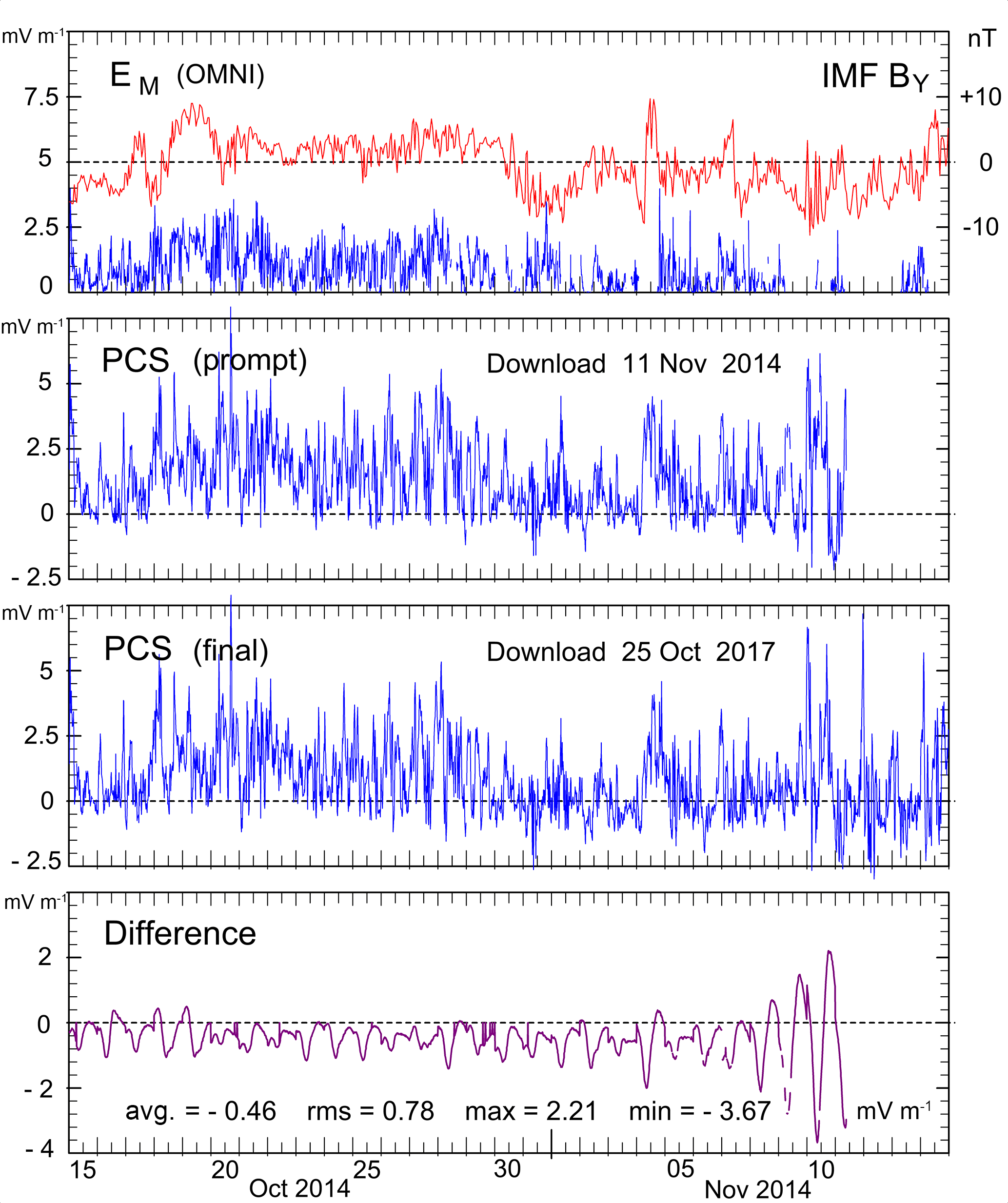
Figure 5From top: solar wind electric field (blue line, left scale) and IMF BY component (red line, right scale), PCS (prompt), PCS (final), and (in bottom panel) differences between final and prompt PCS values. Average, rms, and peak differences are noted. The presented values are 5 min averages of 1 min data.

Figure 6PCS indices for 7 to 11 November 2014 from downloads on 11 November 2014 (red line) and 25 October 2017 (blue line). The prompt values shown by the red curve terminate in the real-time PCS value at the time of download. The displayed values are 5 min averages of the 1 min data.
In Eq. (2) the SS term, FSS, added to derive the quiet level, from which the projected variations, ΔFPROJ, are counted, is a vector comprising the H component (shown in Figs. 1–4) as well as the D component (not presented in J&T2011). With specification of the quiet level defined in Eq. (2), the expression for the PC index in Eq. (1) could be written as
The projection angle varies through 360∘ each day. Hence, the projected term, FSS,PROJ, equals the HSS component in magnitude two times a day (at night and in the day). Thus, the effect on the PC index value can be derived for these two cases (whether real-time or final values) through
The HSS term is derived once a day. With typical daily variations in the slope, α, the ΔPC values at night would be around twice the corresponding values at daytime although the real SS effects are much smaller at night than in daytime (see Fig. 2). Typical values for the slope in June are α=32 nT (mV m−1)−1 at night and α=65 nT (mV m−1)−1 in the day (see http://pcindex.org). Accordingly, the changes in PC index values for differences of 70 nT between the real-time and the final HSS values range between 1.1 mV m−1 in the day and 2.2 mV m−1 with opposite sign at night. Corresponding deviations between real-time and final values of DSS could only increase (not reduce) the amplitudes in the daily oscillations (like those seen in Figs. 5 and 6) of the differences between real-time and final PC index values.
It should be noted that the 3-day median values displayed in Fig. 6b of J&T2011 are possibly smoothed by the authors. At true real-time conditions, the smoothing is not possible for the most recent 3-day median values. Hence, the potential fluctuations might generate still larger excursions in the HSS values and in the derived real-time QL and PC index values than demonstrated here.
Apparently, the real-time PC index values exist only at the time of their presentation at http://pcindex.org. It seems that they are not kept for further analyses of their validity. Hence the only available examples are those recorded at occasional downloads of PC index values. Figure 5 presents an example based on the download of PC indices on 11 November 2014 at 09:41 UT. The data define the prompt PCS index values extending up to the real-time value provided at the time of the download. On the provision that the magnetic data are not changed from their real-time values, the current recalculations with added data turn the prompt PC index data into final values in 1–2 months. The download of final values of PCS for 2014 used here took place on 25 October 2017.
The last value of the PCS (prompt) data in the second panel from the top of Fig. 5 is the real-time value at the time of the download (11 November 2014, 09:41 UT). Further data in this panel are “prompt” values that include the “near-real-time” values. The average, rms, and peak differences between the final and the prompt values for the span of data displayed in Fig. 5 are noted in the bottom panel. It is seen that the prompt values deviate from the final values by up to 3.67 mV m−1 in this example.
Figure 6 holds a more detailed display through the days 7 to 11 November 2014 of the PCS prompt (near-real-time) values (from download 11 November 2014) in the red line and final values (from download 25 October 2017) in the blue line. Note in Fig. 6 that the differences between the final and the prompt PCS values vary between (mostly) positive values at local daytime (local MLT noon at Vostok is at around 13 UT) and negative values at night at twice the amplitude.
The differences between real-time and final values need not be that large. Figure 7 presents PCS values based on the same Vostok magnetic data as those used for the PCS indices displayed in Figs. 5 and 6, but processed according to the methods suggested in Stauning (2016). The quiet reference levels (QLs) for the prompt values from a simulated download on 11 November 2014 were calculated using the “solar rotation weighted” (SRW) QDC method (Stauning, 2011) on Vostok data extending up to the date and time of the download of the PCS values presented in Figs. 5 and 6.
With the SRW method, the QL is constructed by weighted superposition of quiet samples for corresponding times of the day from an interval of ±40 days from the day in question. In the superposition, the samples are weighted to give preference to dates close to (and including) the day in question and to dates with the same view of the sun in its 27-day rotation. In real-time calculations of PC indices, the QL estimates use data recorded 40 days prior to the date and time in question. In post-event calculations, the QL estimates are gradually improved as samples from up to 40 days past the day in question become available. In contrast to the IAGA-endorsed QL method, the SRW method provides adequate QL values at night and preserves the IMF BY-related differences in daytime QL amplitudes (cf. Fig. 2). For QL calculations in real-time applications, the SRW method is inherently more robust to data gaps and other irregularities in the stream of incoming magnetic data than the cubic-spline-based extrapolation method.
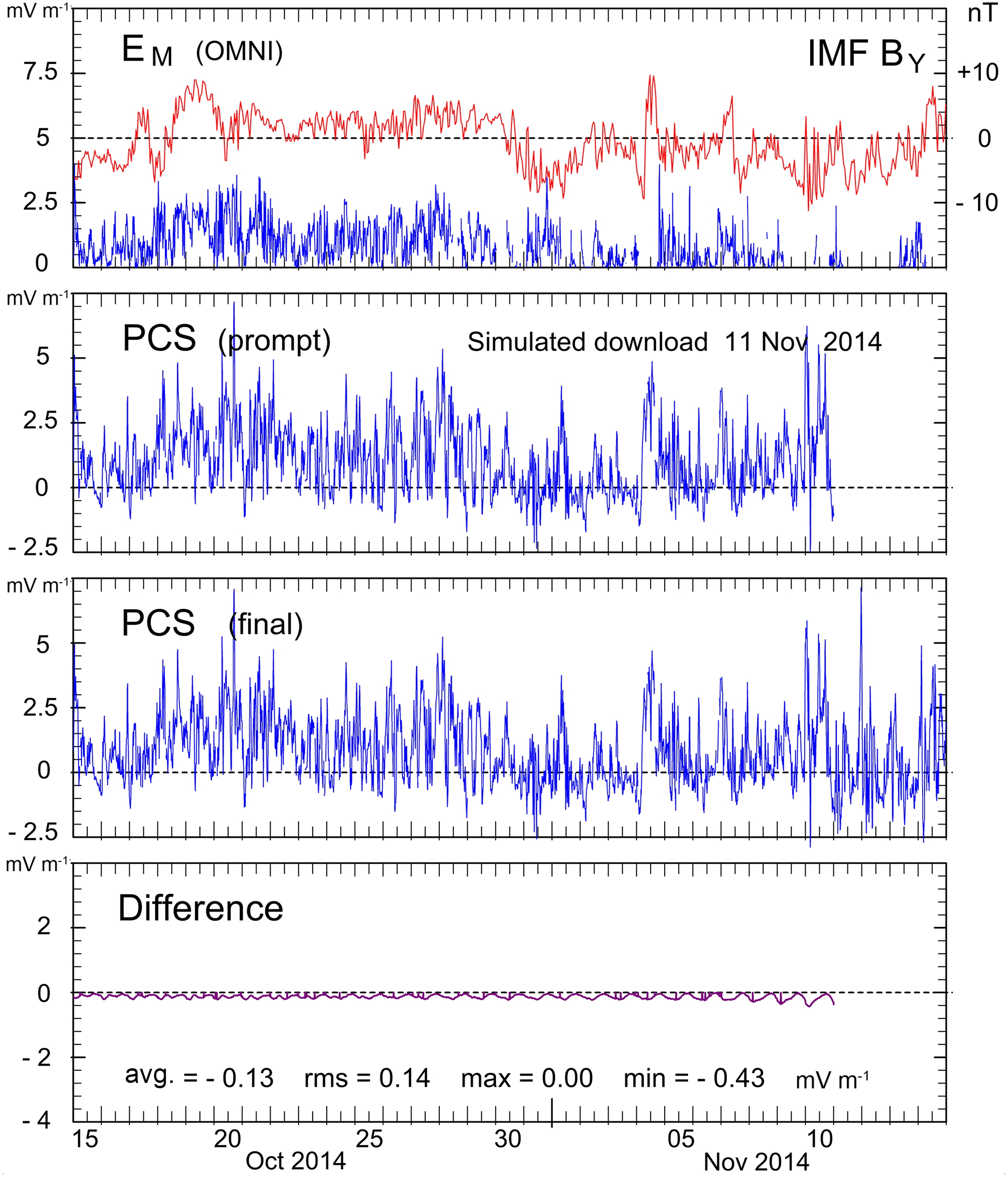
Figure 7Prompt and final PCS index values based on Vostok data for the dates and in the format of Fig. 5. The EM and IMF BY data in the top panel are the same as those presented in Fig. 5. The PCS prompt and final indices have been processed from Vostok data by using the “DMI” methods (Stauning, 2016).
For the case presented in Fig. 7, the maximum difference between prompt and final values is just 0.43 mV m−1. At the start of the interval presented in Fig. 7, the date (15 October) is 27 days from the date (11 November) of simulated download. Thus, just a small part (13/80) of the total amount of samples from the usual ±40 days interval are missing at the start and their weights are low. The derived QDC is now close to its final value. As the date for PC index calculations approaches the simulated download date, more samples ahead of the day in question are missing such that the QDCs may differ more and more from their final values.
The example of large differences between prompt (real-time) and final PC index values presented here in Figs. 5 and 6 agree with the indications presented in Figs. 3 and 4 of the possible effects (large excursions) of using the real-time cubic spline extrapolation to derive the (daily) solar wind sector (SS) term, FSS. In the IAGA-endorsed procedure (Appendix A, 2014), the SS term is part of the quiet reference level, (FQL,SS), from which the magnetic variations included in the PC index calculations are counted (cf. Eq. 2). FQL,SS, furthermore, includes the quiet daily variation, FQDC,SS, calculated around one month earlier and projected forward to the actual date by using past year(s) seasonal trend (J&T2008). The validity of this process is difficult to assess when operating on data corrected for the SS term. The SS effects may not repeat in successive years. However, it is assumed that possible differences between real-time and final FQDC,SS values are relatively small compared to variations in the FSS term.
It should be noted that the example presented in Figs. 5 and 6 just represents one occasional download of PC indices including the real-time value at the time of the download. Further cases not recorded may display still larger deviations between the real-time index values supplied at download times and the final values downloaded at later times and considered to represent the best possible values. The cubic spline extrapolation method to estimate the solar wind sector term for the real-time QLs is vulnerable to the configuration of the four involved 3-day median values, as evident in Figs. 3a–d and 4, and probably also highly sensitive to irregularities in the supply of magnetic data.
The magnitude of the peak differences between prompt and final values found here, ΔPC(max) = 3.67 mV m−1, corresponds to the anticipated PC index levels at strong substorms since PC index values above 2 mV m−1 usually indicate magnetic storm and substorm activity (e.g. Troshichev et al., 2014). Thus, in a real-time monitoring application, the distorted PC index values may indicate ongoing substorm activity during calm conditions or indicate quiet conditions hiding an actual magnetic storm or substorm event.
The present study provides the first reported validity analyses of the IAGA-endorsed method used to generate the quasi-real-time PC index values made available at the web portal http://pcindex.org. It should be noted that the presented and further similar cases are built on occasional downloads of index values. Systematic recordings of the real-time index values supplied from the PC web portal are not available to document the differences between real-time and final PC index values on a comprehensive statistical basis.
-
The inclusion of a solar sector term may change the reference quiet level, particularly at local night, from the level determined from quiet samples recorded during similar IMF BY and seasonal conditions. The aggravated effects by using the real-time procedure to estimate the solar wind sector term by cubic spline forward projection of IMF BY-related variations may cause substantial differences between PC index values determined in real time and those calculated posterior.
-
The observed excessive deviations between real-time and final PC index values agree with expectations based on using here the cubic spline procedure and the example data provided in Janzhura and Troshichev (2011) to determine the solar wind sector terms included in the reference quiet levels (QL) used in the IAGA-endorsed calculations of real-time PC index values.
-
In an example based on the download of PC index data on 11 November 2014, differences between the real-time and later downloaded final PCS index values were found to range up to 3.67 mV m−1, which is at an alarming level considering that PC index values above 2 mV m−1 usually indicate magnetic storm conditions. The example may not even represent the most extreme cases.
-
Results were presented from using different methods (Stauning, 2016) for processing the Vostok data used in the example. Now, the deviations between real-time and final PCS index values were below 0.44 mV m−1. Elements from this procedure, particularly the QL estimate, might be used in possible future modifications of the IAGA-endorsed PC index calculation methods.
Near-real-time PC index values and PCN and PCS index series derived by the IAGA-endorsed procedure are available through the web site: http://pcindex.org. The web site, furthermore, holds PCN and PCS index coefficients. QDC values are not included. The web site includes the document “Polar Cap (PC) Index” (Troshichev, 2011). Prompt and final PCS data used in the present paper are provided in the Supplement.
Geomagnetic data from Qaanaaq and Vostok were supplied from the INTERMAGNET data service center at http://intermagnet.org.
Solar wind OMNI BSN data from combined ACE, WIND, IMP8, and Geotail interplanetary satellite measurements were provided from the OMNIweb data service at the Goddard Space Flight Center, NASA, at http://omniweb.gsfc.nasa.gov
The “DMI” PC index version is documented in the report SR-16-22 (Stauning, 2016) available at the DMI web site: http://www.dmi.dk/fileadmin/user_upload/Rapporter/TR/2016/SR-16-22-PCindex.pdf. Prompt and final PCS values for October–November 2014 calculated by the DMI method are available in the Supplement.
Appendix A (2014): The web site ftp://ftp.space.dtu.dk/WDC/indices/pcn/ includes documentation forwarded to IAGA for endorsement of the PC indices, among others the documents: PC_index_description_main_document.pdf and PC_index_description_Appendix_A.pdf, and a directory, PC_index_description_Appendix_A___file_archive, with program transcripts and data files. The documents referred to in the present work are available in the Supplement.

Figure A1Reproduction of Fig. 6b from Janzhura and Troshichev (2011) referred to in the present Sects. 3 and 4.
-
IAGA PC_index_description_main_document.pdf (12 February 2014)
-
IAGA PC_index_description_appendix_A.pdf (27 January 2014)
-
IAGA PCS October–November 2014 prompt data: pcnpcs2014.zip (download 11 November 2014 09:41)
-
IAGA PCS October–November 2014 final data: pcnpcs2014.zip (download 25 October 2017 11:32)
-
DMI PCS October–November 2014 prompt data: PCS14C.5QP
-
DMI PCS October–November 2014 final data: PCSU2014.5MQ
The supplement related to this article is available online at: https://doi.org/10.5194/angeo-36-621-2018-supplement.
The author declares that he has no conflict of interest.
The staff at the observatories in Qaanaaq and Vostok and their supporting
institutes are gratefully acknowledged for providing high-quality geomagnetic
data for this study. The excellent service at the OMNIweb data center
(http://omniweb.gsfc.nasa.gov) to provide processed solar wind
satellite data, the efficient provision of geomagnetic data from the
INTERMAGNET data center (http://intermagnet.org), and the efficient
performance of the PC index portal (http://pcindex.org) are greatly
appreciated. The author gratefully acknowledges the good collaboration and
many rewarding discussions in the past with Oleg A. Troshichev and
Alexander S. Janzhura at the Arctic and Antarctic Research Institute in St.
Petersburg, Russia.
The topical editor,
Anna Milillo, thanks Alan Rodger for help in evaluating this paper.
Appendix A: available at: ftp://ftp.space.dtu.dk/WDC/indices/pcn/PC_index_IAGA_endorsement_documentation/ (last access: 4 April 2018), 2014.
Friis-Christensen, E., Kamide, Y., Richmond A. D., and Matsushita, S.: Interplanetary magnetic field control of high-latitude electric fields and currents determined from Greenland magnetometer data, J. Geophys. Res., 90, 1325–1338, 1985.
Janzhura, A. S. and Troshichev, O. A.: Determination of the running quiet daily geomagnetic variation, J. Atmos. Sol.-Terr. Phy., 70, 962–972, https://doi.org/10.1016/j.jastp.2007.11.004, 2008.
Janzhura, A. S. and Troshichev, O. A.: Identification of the IMF sector structure in near-real time by ground magnetic data, Ann. Geophys., 29, 1491–1500, https://doi.org/10.5194/angeo-29-1491-2011, 2011.
Stauning, P.: Determination of the quiet daily geomagnetic variations for polar regions, J. Atm. Sol.-Terr. Phy., 73, 2314–2330, https://doi.org/10.1016/j.jastp.2011.07.004, 2011.
Stauning, P.: The Polar Cap index: A critical review of methods and a new approach, J. Geophys. Res.-Space, 118, 5021–5038, https://doi.org/10.1002/jgra.50462, 2013a.
Stauning, P.: Comments on quiet daily variation derivation in “Identification of the IMF sector structure in near-real time by ground magnetic data” by Janzhura and Troshichev (2011), Ann. Geophys., 31, 1221–1225, https://doi.org/10.5194/angeo-31-1221-2013, 2013b.
Stauning, P.: A critical note on the IAGA-endorsed Polar Cap index procedure: effects of solar wind sector structure and reverse polar convection, Ann. Geophys., 33, 1443–1455, https://doi.org/10.5194/angeo-33-1443-2015, 2015.
Stauning, P.: The Polar Cap (PC) Index: Derivation Procedures and Quality Control, DMI Scientific Report SR-16-22, available at: http://www.dmi.dk/fileadmin/user_upload/Rapporter/TR/2016/SR-16-22-PCindex.pdf (last access: 4 April 2018), 2016.
Svalgaard, L.: Polar cap magnetic variations and their relationship with the interplanetary magnetic sector structure, J. Geophys. Res. 78, 2064–2078, 1973.
Troshichev, O. A.: Polar Cap (PC) Index, available at: http://pcindex.org or at: http://geophys.aari.ru/Description.pdf (last access: 4 April 2018), 2011.
Troshichev, O. A. and Janzhura, A.: Space Weather monitoring by ground-based means, Springer Praxis Books, Heidelberg, https://doi.org/10.1007/978-3-642-16803-1, 2012.
Troshichev, O. A., Janzhura, A. S., and Stauning, P.: Unified PCN and PCS indices: method of calculation, physical sense and dependence on the IMF azimuthal and northward components, J. Geophys. Res., 111, A05208, https://doi.org/10.1029/2005JA011402, 2006.
Troshichev, O. A., Podorozhkina, N. A., Sormakov, D. A., and Janzhura, A. S.: PC index as a proxy of the solar wind energy that entered into the magnetosphere: 1. Development of magnetic substorms, J. Geophys. Res.-Space, 119, 6521–6540, https://doi.org/10.1002/2014JA019940, 2014.
- Abstract
- Introduction
- Quiet reference level and solar wind sector term
- Derivation of the solar wind sector term in real time
- Recorded differences between the real-time and final PC index values
- Different PC index versions
- Summary
- Conclusions
- Data availability
- Appendix A
- Information about the Supplement
- Competing interests
- Acknowledgements
- References
- Supplement