The three Swarm satellites were launched into a polar low-Earth orbit (LEO) on 22 November 2013. During the commissioning phase the three satellites flew on the same orbit, following each other with an increasing separation. Since 17 April 2014 Swarm A and C have orbited side-by-side (1.4^∘ east–west separation) at 460 km altitude and an inclination of 87.4^∘, while Swarm B orbits at 510 km altitude and an inclination of 87.8^∘. The orbital planes of Swarm B relative to A and C drift away slowly (by 5–6 min day⁻¹) in magnetic local time (MLT) due to the different inclinations. In this study we utilized the FAC data derived from vector magnetic field data recorded by the fluxgate magnetometers with a resolution of 10 pT between 1 January 2014 and 31 December 2017. By the end of the investigated interval the MLT separation between Swarm A and B increased to ∼ 6 h. For inter-satellite comparisons Swarm A is preferred over Swarm C in this study, since the absolute scalar magnetometer instrument on the latter stopped working on 5 November 2014, resulting in a somewhat poorer calibration. However, we found no significant difference in the performance of Swarm A and C in monitoring the plasmapause.

Our plasmapause detection method is based on the localization of the equatorward boundary of SSFAC activity deduced from the transverse toroidal component of the geomagnetic field fluctuations observed at LEO. This new tool, which yields unprecedented details on the dynamic behaviour of the plasmapause, was first introduced and described in detail by Heilig and Lühr (2013).

For validation purposes we used in situ plasma density data. The twin (A and B) VAP spacecraft were launched on 30 August 2012 into a highly elliptical (with perigee at 700 km, apogee at 5.8 R_E, orbital period ∼ 9 h), low inclination orbit with the primary objective of studying the Earth's Van Allen radiation belts. The in situ electron density data used in this study are inferred from the upper hybrid resonance frequency f_uh observations by the plasma wave High Frequency Receiver (Waves HFR) instrument of the Electric and Magnetic Field Instrument Suite and Integrated Science (EMFISIS) suite. We used the electron number densities N_e observed between 1 January 2014 and 1 July 2016 by VAP A as derived by Zhelavskaya et al. (2016) through the Neural-network-based Upper hybrid Resonance Determination (NURD) algorithm. These in situ electron density data are openly available at the ftp://rbm.epss.ucla.edu/ftpdisk1/NURD/ ftp site. The NURD dataset includes L and geomagnetic latitude Λ along with density values. The spatial resolution in L ranges from a few 0.0001 R_E at low L to a few 0.001 R_E at high L. At such a narrow spacing the measurement error can easily exceed the true change rates, making the calculated density gradients very noisy. In order to decrease this effect, density profiles were filtered by applying a 31-point moving average. The length of the filter corresponds to L-value ranges of 0.001–0.1 R_E, long enough to sufficiently depress the noise, but short enough not to affect the location of the PP associated density gradient significantly. After filtering, density profiles were down-sampled at dL = 0.01 R_E resolution. From the resampled density values we determined orbit-by-orbit the PP position as the earthward edge of the innermost density gradient exceeding a factor of 5 drop within dL = 0.25 R_E. We note that the gradient threshold we applied is twice as large as those applied by previous authors, simply because we found that the old (lower) threshold in many cases identifies the PP inward from the clear sharpest drops. This difference stems from the different spatial resolution between old and new data. The lower resolution of data from previous missions heavily smoothed the density profiles, necessitating the use of a lower threshold for PP detection. For better consistency with earlier data, we also calculated the neighbourhood of the previously described innermost sharp gradient, where the density gradient exceeds a factor of 5 drop within dL = 0.5 R_E, i.e. the traditional threshold. The lower limit of this interval is then chosen as the location of the PP.

We also note that the VAP PP positions were derived from in situ density observations made at low latitudes. Since the detection relies on relative changes across L-shells, there is no significant impact of this choice on the results. This can be easily seen by combining the field-aligned distribution of plasmaspheric electron density $\frac{N_{\mathrm{e}}}{N_{\mathrm{e}\mathrm{0}}}=\frac{r_{\mathrm{0}}}{r}$, where N_e0 is the equatorial density, r₀ is the radial distance of the equatorial point of the field line, r is the radial distance (Denton et al., 2006), and the equation of a dipole field line is r=r₀cos ²Λ. From these we get $\frac{N_{\mathrm{e}}\left({\mathrm{\Lambda }}_{\mathrm{1}}\right)}{N_{\mathrm{e}}\left({\mathrm{\Lambda }}_{\mathrm{2}}\right)}=\frac{{\cos }^{\mathrm{2}}{\mathrm{\Lambda }}_{\mathrm{2}}}{{\cos }^{\mathrm{2}}{\mathrm{\Lambda }}_{\mathrm{1}}}$ for the ratio of the densities at two points along the field line. In the vicinity of the geomagnetic equator ($\mathrm{\Lambda }<{\mathrm{30}}^{\circ })$ for closely separated (ΔΛ < 3^∘) points, this formula yields only a few percent difference in N_e that is negligible compared to the factor of 5 drop we look for. Hereafter, VAP observed PP will be referred to as PP_N_e to distinguish them from the SSFAC index derived from Swarm FAC observations.

The main steps of data processing applied to Swarm observations are as follows. First, the field-aligned current (FAC) density, $j_{//}$, available as the Swarm Level 2 product FACxTMS_2F (where x stands for A, B or C identifying the satellite) for each satellite individually, is high-pass filtered by a third-order Butterworth with a −3 dB cut-off at 250 mHz. The chosen cut-off frequency ensuring precise boundary localization corresponds to a ∼ 30 km spatial scale along the (quasi-meridional) orbit. Then the logarithm of the squared SSFAC density (in units µA m⁻²) is taken, and a boxcar averaging is applied to derive the SSFAC power level, S, subsequently used as a detection signal:

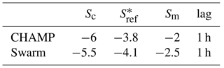
The detection of the SSFAC inner (equatorward) boundary is a multistep process. As a first step, each orbit is divided into four orbital segments including data from the magnetic equator to the poles. Then all segments are scanned for the innermost transition of S between two pre-defined reference levels (an increase in S from $S_{\mathrm{c}}=-\mathrm{5.5}$ to $S_{\mathrm{m}}=-\mathrm{2.5})$. The applied reference values are found typically only inside/outside the nominal plasmapause (here the nominal plasmapause locations are derived from the Kp-based model of O'Brien and Moldwin, 2003). The L-values related to the corresponding S reference levels are denoted by L_c and L_m, respectively, where the L-value is calculated from the modified apex magnetic latitude assuming a dipole field geometry ($L=r_{\mathrm{ref}}/{\cos }^{\mathrm{2}}\left(\mathrm{mlat}\right))$, where  r_ref≈1.02 is the geocentric distance of the E-region as reference height (110 km) in Earth's radii (6371.2 km). In the next step the change in the SSFAC power level within the transition zone [L_c; L_m] is represented by a linear fit, $S^{\ast }=aL+b$, and σ, the RMS value of the residuals ($S-S^{\ast })$ in the [L_c;  L_m] interval, is calculated. The width of the boundary dL is defined as L_c−L_m. Finally, the L-value where S^∗ equals a threshold reference level, $S_{\mathrm{ref}}^{\ast }$ (∼ −4.0), is taken as the position of the boundary, L_ssfac. Whenever L_ssfac lies outside the interval [L_c; L_m], it is rejected. This typically happens when the boundary is not well defined, mostly on the dayside. The resulting detection of the equatorward boundary of intense SSFACs (the SSFAC index) is related to the L-value of the plasmapause in units of Earth radii (R_E). The fit quality parameters, dL (the boundary width) and σ (characterizing the quality of the fit), are used to exclude less-defined transitions similarly as described in Heilig and Lühr (2013). The detection parameters (reference levels) applied at Swarm data analysis, and for comparison also for CHAMP, are given in Table 1.

Table 1Detection parameters applied for CHAMP and Swarm data.

Download Print Version | Download XLSX

To optimize the quality of the detection results, a fine adjustment of the reference value $S_{\mathrm{ref}}^{\ast }$ is needed. Following Heilig and Lühr (2013) we did it by maximizing the absolute correlation strength between the boundary position, L_ssfac, and the geomagnetic index Kp. Allowing for comparisons on shorter timescales than the 3 h cadence of Kp, the Kp index was linearly interpolated at UTs of the SSFAC index. The best correlation was found at $S_{\mathrm{ref}}^{\ast }=$ −4.1 (corresponding to ∼ 0.01 µA m⁻² SSFAC density), very close to the value found for CHAMP (Table 1, Fig. 1b). During this and further calculations, Kp was delayed in time by 1 h. This value is inferred from a cross-correlation analysis between Kp and L_ssfac (Fig. 1a), and corresponds to the mean response time of the boundary to changes in geomagnetic activity.

Figure 1(a) L_ssfac–Kp cross-correlation, and (b) correlation between L_ssfac and Kp as a function of the reference level $S_{\mathrm{ref}}^{\ast }$.

Download

To check whether the SSFAC boundary behaves similarly as the PP_N_e does, we investigated how the SSFAC index depends on the time history of Kp. For the correlation analysis, we determined the peak Kp in an x hour (x varies from 0 to 12 h) long interval ending y hours before (y varies from −6 to 2 h at 0.5 h steps) the investigated event, i.e. if the event time is depicted by t₀, the considered interval is [$t_{\mathrm{0}}+y-x;t_{\mathrm{0}}+y$]. The SSFAC indices (L_ssfac boundary positions) are correlated with the interval peak Kps. The result of this analysis is summarized in Fig. 2a and b. The individual columns of these figures can be read as cross-correlations between the SSFAC index and Kp_max as a function of the interval length.

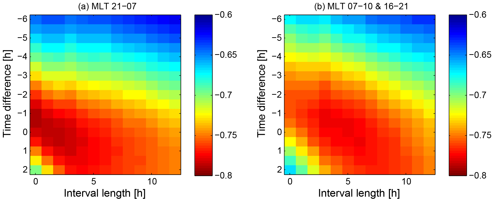
Figure 2Correlation strength between the SSFAC index and the peak Kp as a function of the length of the interval (horizontal axis), where the peak Kp is taken from the time difference (vertical axis) between the end of the interval and SSFAC index observation (a) in the sector (MLT 21:00–07:00), and (b) for morning (MLT: 07:00–10:00) and evening (MLT: 16:00—21:00) hours.

Download

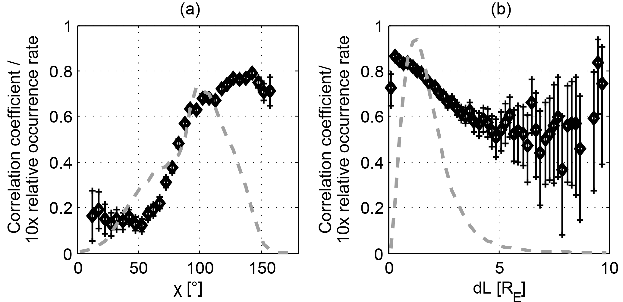
Figure 3(a) Dependence of the L_ssfac–Kp correlation on the solar zenith angle “χ” while “dL” < 3 (diamonds) with 95 % confidence intervals (vertical lines) along with 10 times the relative occurrence rate of “χ” values (dashed line), and (b) the same correlation/occurrence rates in the same format as in (a) but as a function of the boundary width “dL” while χ > 90^∘.

Download

Similar correlation matrices were calculated separately for all the 24:00 MLT sectors (0..1, 1..2, 2..3, etc., not shown). We identified two distinct behaviours. On the night side (21:00–07:00 MLT) the response of the boundary is slightly faster than on the morning and dusk (07:00–10:00 and 16:00–21:00 MLT) sides. The variation of the boundary positions follows quite tightly any changes in Kp, with an average response time of 0.5–1 h (i.e. time difference or lag is between −0.5 and −1 h) in both Fig. 2a (night side case: 21:00–07:00 MLT) and b (07:00–10:00 and 16:00–21:00 MLT). Positive lag is unphysical and can be attributed to the low (3 h) time resolution of Kp. The interval length yielding the strongest correlation (deepest red) depends on the lag. The absolute maximum on the night side/dayside is found at −1/−1 h lag and 0/3–4 h interval length, respectively, meaning that the SSFAC index is dependent mainly on the latest/latest two values of Kp. Nighttime response is practically immediate, and even on the dayside the memory of the SSFAC index does not exceed a few hours.

The observation that the ∼ 1 h response time does not seem to depend on MLT can be interpreted as a synchronous response of the whole boundary to changes in geomagnetic activity. It means that the behaviour of the SSFAC index is different from that of the PP_N_e, which shows a local time dependent response time to magnetic activity (Katus et al., 2015; Zhang et al., 2017).

The correlation strength between the SSFAC index and Kp was found by Heilig and Lühr (2013) to vary with MLT, solar zenith angle χ, and the fit quality parameters. We repeated this analysis with Swarm data and the results confirm our previous findings: the correlation is stronger than 0.6 during nighttime conditions (χ > 90^∘) (Fig. 3a) or between 18:00 and 06:00 MLT. On the dayside, the detection of the boundary is disturbed by other phenomena, such as shear Alfvén waves including geomagnetic field line resonances (Heilig et al., 2013). As another example, Fig. 3b clearly presents the decrease in the correlation strength with increasing boundary width, dL. The correlation is stronger than 0.65 for steeper slopes (“a” > 0.5 or dL < 3) on the night side. This finding suggests that the boundary can be detected easier and more accurately, when the boundary is sharper. This happens, as we will see, during increased geomagnetic activity.

Figure 4(a) Kp, (b) Dst, and (c) log(AE) dependence of the SSFAC index.

Download

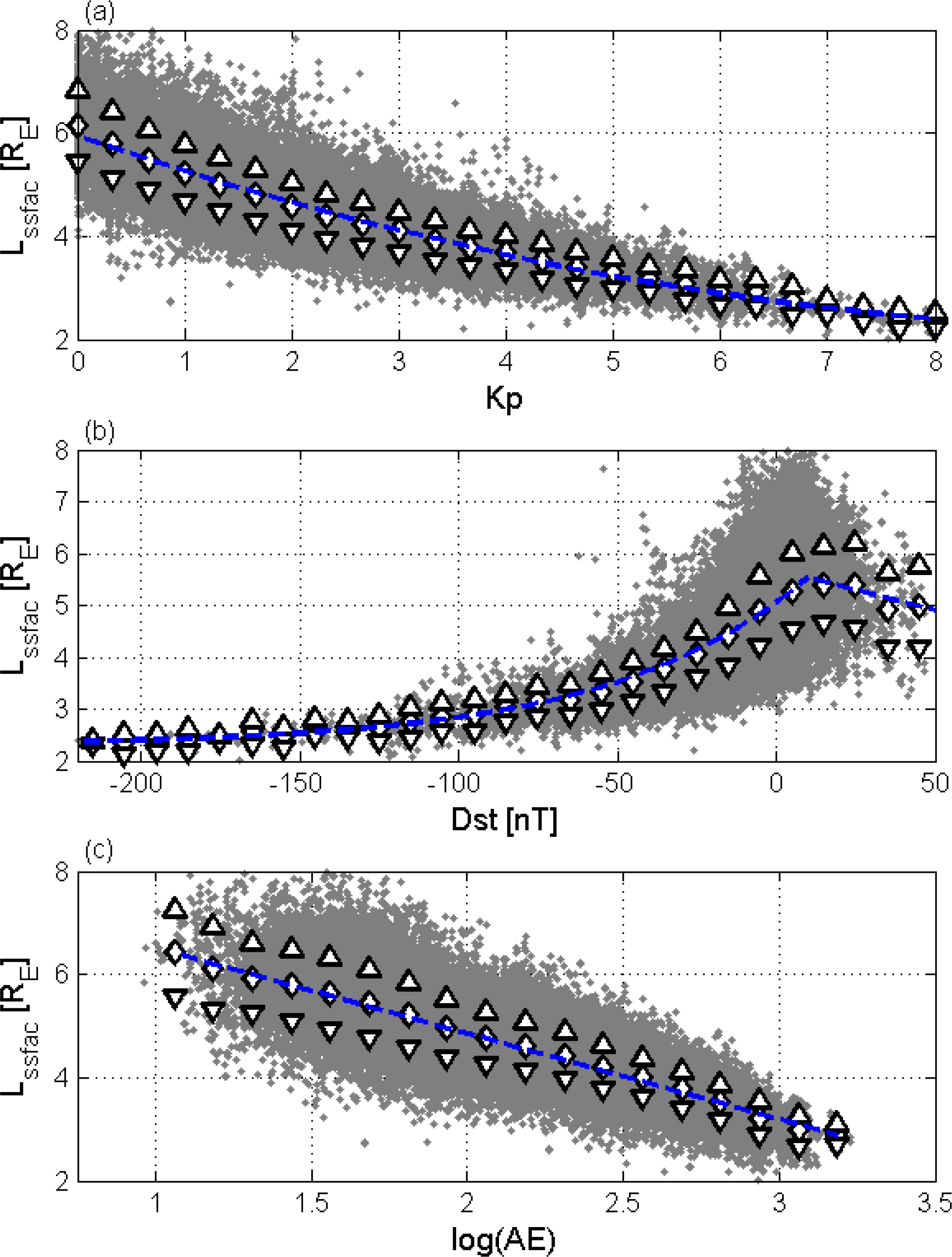
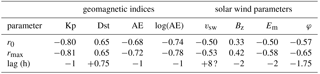
In the following, based on the above and previous (Heilig and Lühr, 2013) findings, our statistical analysis of the SSFAC index is restricted to sharp (dL < 3) boundary transitions observed at solar zenith angles χ greater than 90^∘ and between 18:00 and 06:00 MLT. These conditions reduce the overall 242 317 boundary crossings to 84 010 (35 % of all crossings). Outliers standing out more than 0.5 R_E from the five-point running mean are then removed, reducing further the event number to 68 344 suitable observations (28 % of all crossings). For the different magnetic activity indices Kp, Dst, AE, and log(AE) the cross-correlation maximizes at r_max for the lag times: −0.81 at −1 h lag (Fig. 4a), 0.65 at +0.75 h lag (Fig. 4b), −0.72 at −1 h lag, and −0.78 at −1 h lag (Fig. 4c), respectively (see Table 2 for a summary). This confirms that Kp describes best the average behaviour and the dynamics of the boundary. That is why we used Kp for deriving an empirical model. However, it is still worth having a closer look at the dependences of all the indices.

Table 2Summary of cross-correlation analyses between the SSFAC index and the considered parameters.

Download Print Version | Download XLSX

The Kp dependence (time-shifted) can be approximated quite well by a simple ratic function (Fig. 4a, Eq. 2), similar to that of Heilig and Lühr (2013):

In Fig. 4a, and also in the following plots, triangles depict the mean ± standard deviation values. The correlation strength between the observations and the Kp-based model is 0.81. As Fig. 4b shows, unlike the Kp dependence, the Dst index does not influence the SSFAC index evenly over its full range, mainly when Dst is negative, i.e. during the storm-time intensified ring current. For these values Eq. (3) presents an exponential fit accounting for the dependence. At the same time, positive Dst values typically occurring during the initial phase of geomagnetic storms as a consequence of the magnetopause current increase do not seem to have a strong impact. A possible reason is that while the ring current is involved in the processes forming the new PP, the magnetopause current does not.

The relation to the AE index is shown in Fig. 4c. An improved linear dependence of the SSFAC index location was found for log(AE) (Eq. 4). Unlike the Dst, a monotone dependence extends over the full range of the AE index, indicating that auroral electrojets of any strength correlate with the SSFAC boundary position.

While the SSFAC boundary is observed both below L= 2 and beyond L= 8, none of the above index-based models can account for the whole range of variations. The output of the Kp-based model ranges from L= 2.3 (Kp = 9) to L= 6.0 (Kp = 0). The Dst-based model estimates vary between L= 2.3 (Dst = −500 nT) and L= 5.7 (Dst = 10 nT), while the AE model yields values between L= 2.9 (AE = 1600 nT) and L= 6.5 (AE = 10 nT). In all three cases the range of L variation accounted for by the model is nearly the same, ΔL= 3.5; however, the baselines are different. The Dst/AE-based model is capable of accounting for the lowest/highest extremes, respectively. From the stronger correlation and the 1 h response time it seems that the AE index (strength of the auroral electrojet) reflects more closely the processes that form the SSFAC boundary than the Dst index. At the same time, large Dst indices (developed ring current) tend to be concomitant with the inward motion of the SSFAC boundary below the L_ssfac=3 limit. Indeed, during intense storms, when $\mathrm{Dst}<-\mathrm{100}\mathrm{nT}$, L_ssfac stays below 3 R_E.

Since the geomagnetic activity is driven by Sun–Earth interactions, and the plasmapause location is controlled to first approximation by the magnetospheric convection, it is not surprising that there is a link between the SSFAC equatorward boundary and some interplanetary parameters accounting for the solar-wind–magnetosphere coupling, as well. We found a negative correlation (Table 2) with the solar wind speed (v_sw), a weak positive correlation with the IMF GSM southward component (B_z), and again negative correlations with two solar-wind–magnetospheric coupling parameters: the merging electric field (Kan and Lee, 1979) $E_{\mathrm{m}}=v_{\mathrm{sw}}{B}_t{\sin }^{\mathrm{2}}\frac{\mathit{\theta }}{\mathrm{2}}$, and the coupling parameter $\mathit{\phi }=v_{\mathrm{sw}}B{\sin }^{\mathrm{2}}\frac{\mathit{\theta }}{\mathrm{2}}$ suggested by Larsen et al. (2007). Here B_t ∕ B is the IMF component perpendicular to the Sun–Earth line/the total IMF, respectively, and θ is the clock angle, i.e. the angle between B_t and B_z. Although the merging proxies give higher coefficients (−0.58 and −0.65), these are still weaker than the correlations with geomagnetic indices. Moreover, the time lags are typically 2 h, twice as large as for the Kp and AE indices. These are likely because of the less direct link between the SSFAC boundary dynamics and the solar wind conditions, compared to the more direct impact of the auroral dynamics and the ring current. We note here that the positive time lag found for solar wind speed is unphysical and was neglected during further analysis. Solar wind speed mostly changes on longer timescales than plasmasphere dynamics and that is why the cross-correlation peak is rather flat, as can be seen from the similar correlation strength at +8 h (−0.53) and at 0 h time lag (−0.50) in Table 2. This makes the determination of the response time less reliable.

The nature of the dependence of the boundary location on the considered four solar wind parameters can be seen in Fig. 5a–d. Functional dependences are given by Eqs. (5) to (8). As shown in Fig. 5b, B_z has a significant influence only when it is southward (negative), i.e. when dayside IMF-geomagnetic field line merging takes place, a process that drives magnetospheric convection. The merging electric field E_m and the coupling parameter φ are even more directly linked to magnetospheric convection. It is known that the convection plays a crucial role in the formation of the plasmapause. Whenever the convection increases, the plasmasphere shrinks.

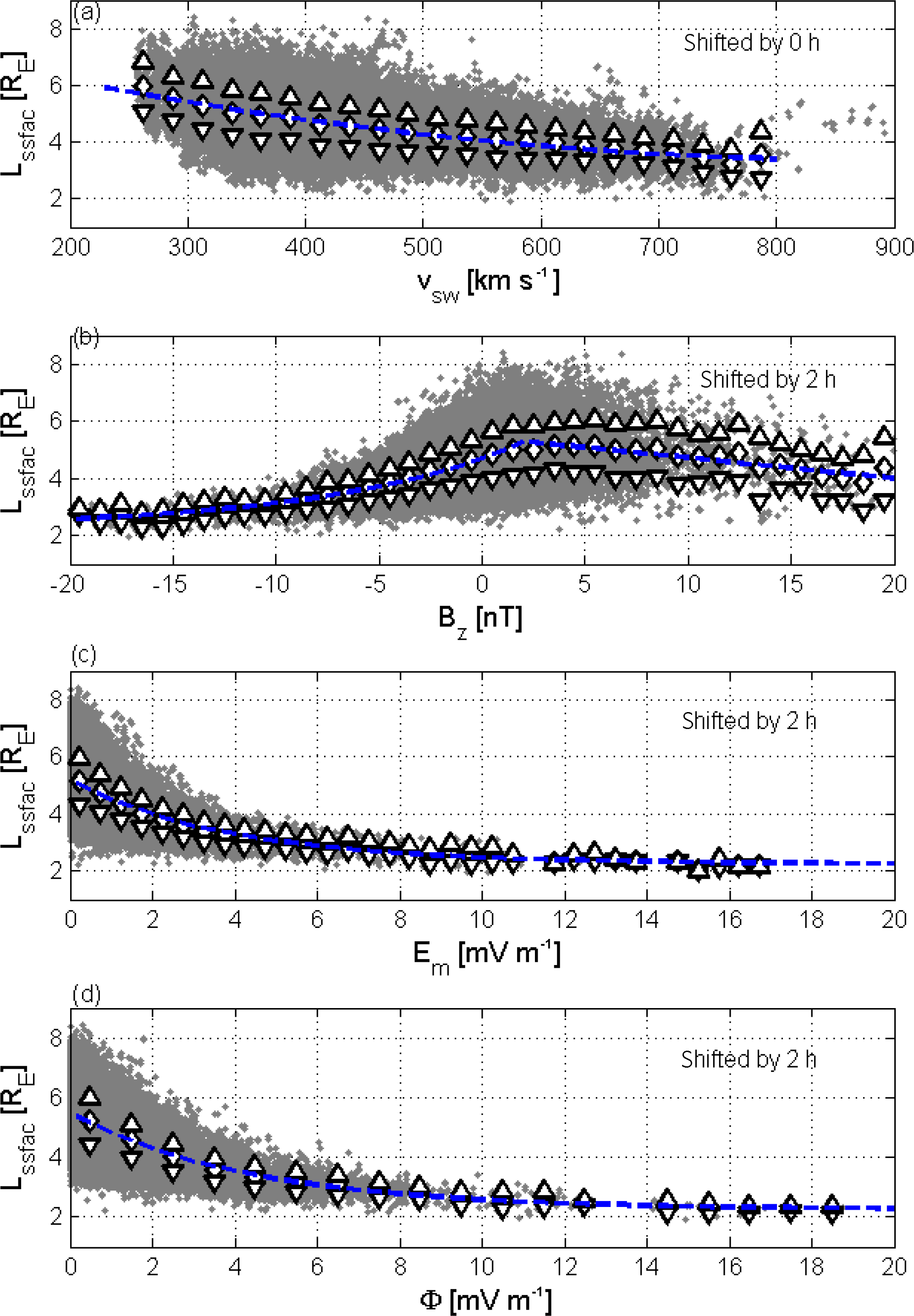
Figure 5Dependence of the SSFAC index on the (a) solar wind speed, (b) B_z IMF south GSM component, (c) merging electric field, and (d) coupling parameter φ.

Download

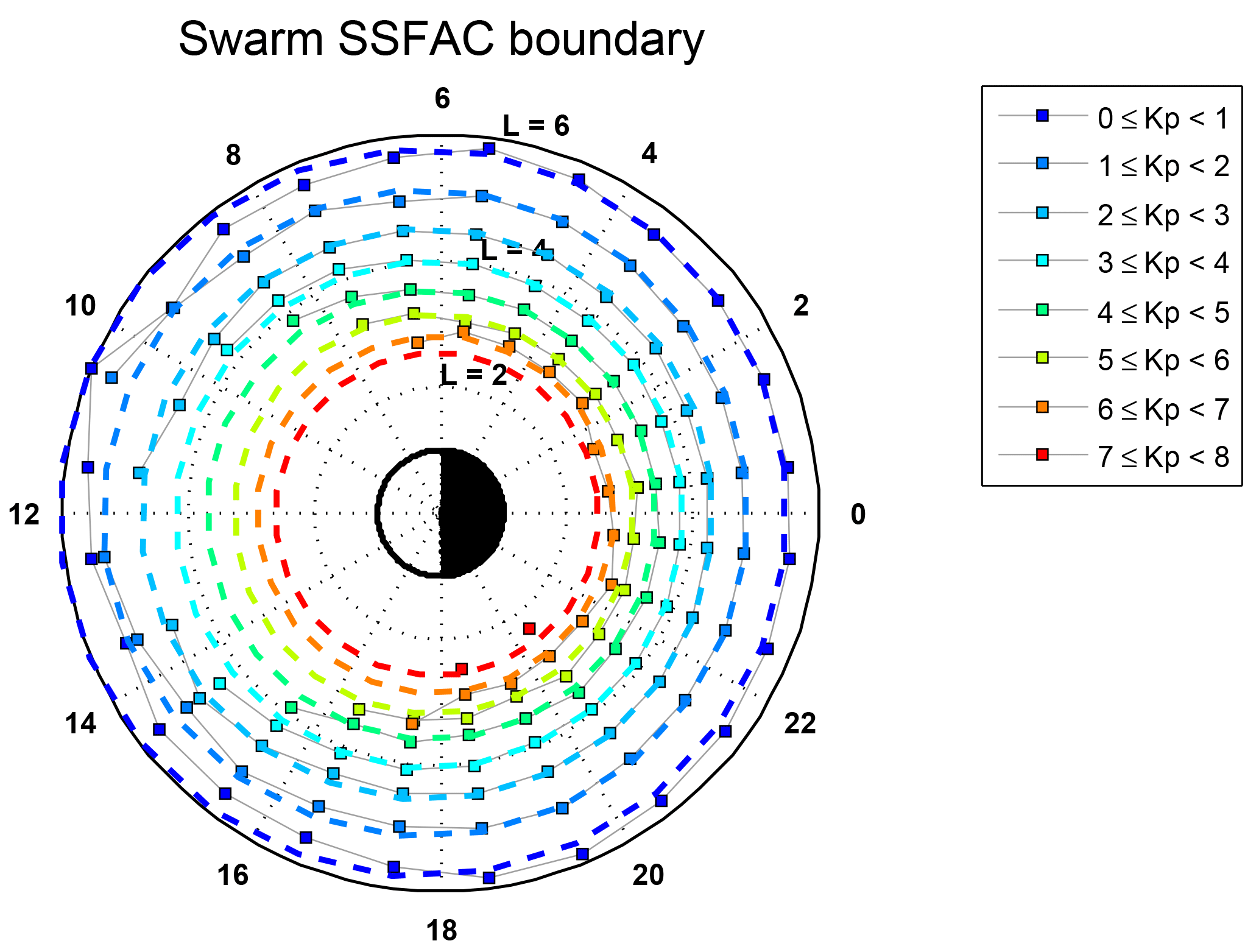
Before starting to discuss the dynamics of the plasmapause we have a detailed look at the small-scale FAC boundary. In Fig. 6 the mean L-values of the SSFAC inner boundary calculated from all observations between 1 January 2014 and 31 December 2017 from all three Swarm satellites are presented on a dial plot as a function of MLT. Individual circles are drawn for different levels of geomagnetic activity ($\mathrm{0}\le \mathrm{Kp}<\mathrm{1}$, $\mathrm{1}\le \mathrm{Kp}<\mathrm{2}$, $\mathrm{2}\le \mathrm{Kp}<\mathrm{3}$, etc.), while the polar histogram in the bottom right presents the MLT distribution of the sample numbers. Only the mean positions of the boundary are shown, where at least 10 observations are available. For the above-mentioned reasons, the detection is restricted to times when χ > 90^∘, causing the asymmetric day–night MLT distribution of detections (see histogram). This is also the main reason for the dayside gap in the boundary determination, especially at high Kp.

The shape of the boundary in Fig. 6 closely resembles a circle in L versus MLT space for any level of geomagnetic activity. The radius of the circle scales inversely with Kp. The circles are not exactly geocentric, and the centres are slightly shifted toward noon. The standard deviation of the individual L_ssfac observations is also a clear function of Kp, decreasing from ∼0.7 R_E at Kp = 0 to ∼0.2 R_E at Kp = 7; however, it hardly depends on MLT. The uncertainty of the means (SD ∕ sqrt(N)) is 0.01–0.02 R_E at each Kp level.

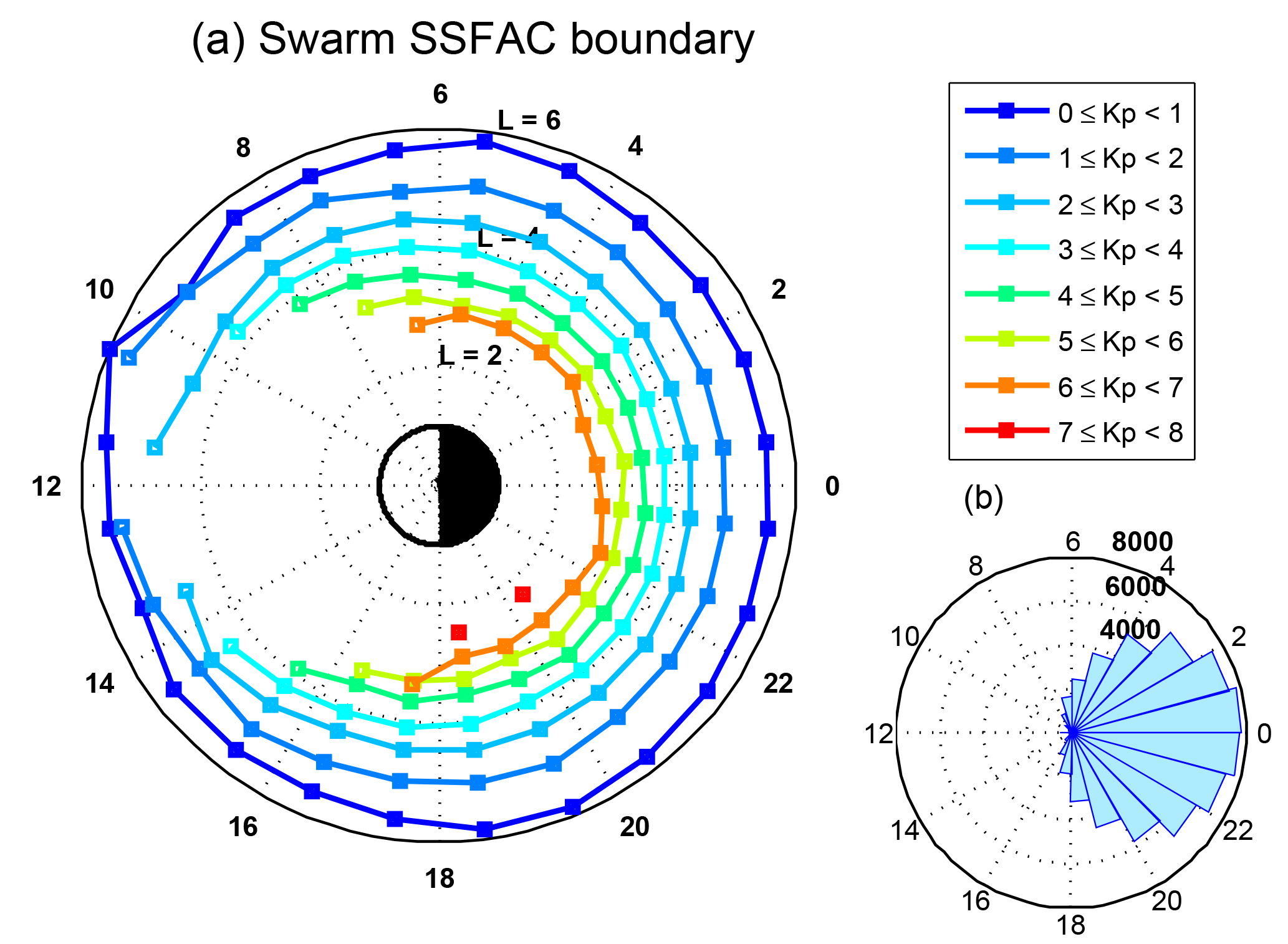
Figure 6(a) Mean boundary positions as a function of MLT at different levels of Kp (0–1, 1–2, 2–3, 3–4, 4–5, 5–6, 6–7, 7–8) and (b) the MLT distribution of the boundary crossings.

Download

Figure 7Average width of the transition zone (dL) as a function of Kp (χ > 90^∘).

Download

Not only the boundary position, but also the boundary width, is a function of Kp. The boundary gets narrower when geomagnetic activity increases, as shown in Fig. 7. At low activity, the mean width is around 2.5 R_E, but the scatter is large, while for Kp > 6 the boundary becomes narrower than 1 R_E. The overwhelming majority of the boundary observations are made at relatively sharp boundaries, i.e. when the boundary width is lower than 3 R_E (see Fig. 3b). As stated before, in our statistical analysis only these sharper boundaries were considered.

For a given level of Kp, we model the observed boundary in L space by an eccentric circle. The position of a point P on the circle is given by its polar coordinates L_mod and $\mathit{\phi }=\mathrm{2}\mathit{\pi }\mathrm{MLT}/\mathrm{24}$ as shown in Fig. 8. If the circle is centred at C(c,φ_c) and has a radius R, L_mod can be derived for any MLT by applying the formula

where d$\mathit{\phi }=\mathrm{2}\mathit{\pi }\left(\left(\mathrm{MLT}-{\mathrm{MLT}}_{\mathrm{c}}\right)/\mathrm{24}\right)$ and ${\mathrm{MLT}}_{\mathrm{c}}=\mathrm{24}\mathrm{h}\cdot {\mathit{\phi }}_{\mathrm{c}}/$360^∘.

Figure 8Sketch of the applied model for a fixed level of geomagnetic activity.

Download

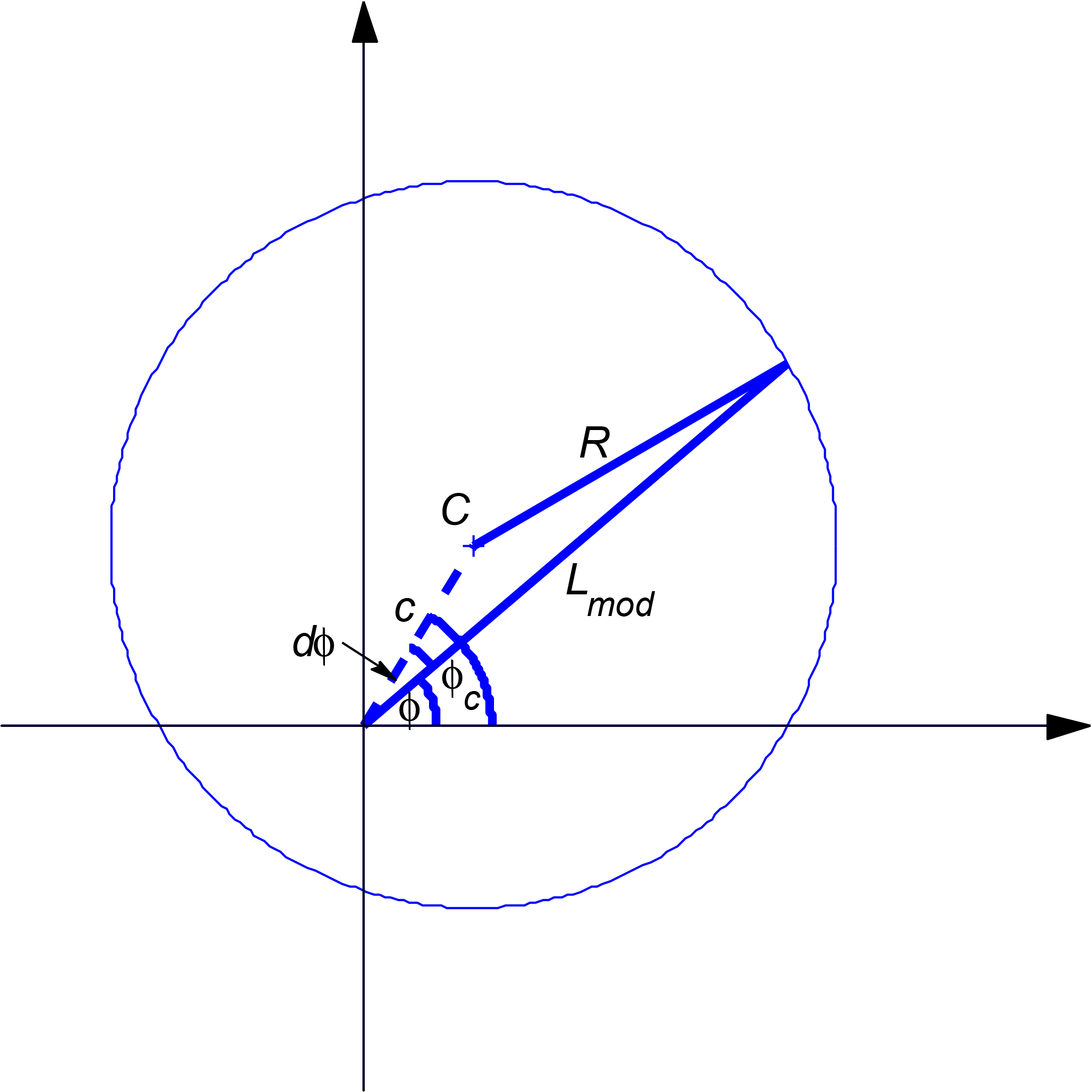
Moreover, we suppose that the position of C and the radius of the circle R have a linear/ratic dependence on Kp, respectively, that is

where c₀ and MLT₀ define the position of the centre and R₀ is the radius of the circle, both at Kp=0, while p₁, p₂, γ_c, γ_mlt are free model parameters. Based on 68344 boundary positions observed during the period 1 January 2014–31 December 2017, the following model parameters (with 95 % confidence bounds) were obtained:

The corresponding model is presented in Fig. 9 as dashed circular curves. The centres of the circulars hardly move with increasing Kp. From Kp = 0 to Kp = 6, it moves from MLT_c= 12.2, c= 0.3 R_E to MLT_c= 13.4, c=0.1 R_E. The mean residuals (observation–model) in each bin are between −0.3 and 0.2 R_E at all Kp levels between 1 and 6. At Kp = 0 the mean residuals are in the range −0.6–0.2 R_E.

Figure 9Empirical model of the inner SSFAC boundary.

Download

Any of the three Swarm satellites visits all the MLT sectors during every 132-day period. Five full years of data are needed for an even coverage of local time during all seasons. Since we consider only 4 years, our model might suffer from a seasonal bias. We found, however, that the seasonal variation is small (±0.13 R_E or ±3 %) and dominantly caused by the varying geomagnetic conditions (not shown). Therefore no significant improvements in seasonal specification are expected by considering slightly longer datasets from Swarm.

4.1 Extension of L_ssfac observed at some MLT to any other MLT

The model derived in the previous section can be used in various ways. First, it can be used as a climatology model. When no boundary observations are available, L_mod can be calculated directly from MLT and Kp as inputs. However, if we have an observation of L_ssfac=L_obs at a certain MLT_obs and the geomagnetic activity given by the Kp index is known, we can, by combining the model (yielding the shape and the centre of the boundary) with the actual observation (providing the actual radius), estimate L_ssfac at any other MLT. This is done by rescaling the size of the boundary based on the actual observation, while taking the average circular shape and Kp-dependent centre position from the model:

$$\begin{array}{}\text{(11)}& R^{\prime }=\sqrt{L_{\mathrm{obs}}^{\mathrm{2}}+c^{\mathrm{2}}-\mathrm{2}c{L}_{\mathrm{obs}}\cos \mathrm{d}{\mathit{\phi }}_{\mathrm{obs}}}.\end{array}$$

Since the Kp dependence of both c and MLT_c is found to be very weak, we can regard them as constant, e.g. $c=\mathrm{0.2}{R}_{\mathrm{E}},{\mathrm{MLT}}_{\mathrm{c}}=$ 12 h, while d${\mathit{\phi }}_{\mathrm{obs}}=\mathrm{2}\mathit{\pi }\left(\frac{\left({\mathrm{MLT}}_{\mathrm{obs}}-{\mathrm{MLT}}_{\mathrm{c}}\right)}{\mathrm{24}\mathrm{h}}\right)=\mathit{\pi }\left(\frac{{\mathrm{MLT}}_{\mathrm{obs}}}{\mathrm{12}\mathrm{h}}-\mathrm{1}\right)$ can be calculated from the model. This will cause less than 0.05 R_E error. Now L_mod at any MLT can be computed by the direct use of Eq. (9), but substituting R^′ into R.

We verified our SSFAC index estimates by checking the consistency between the observations of the different satellites. By using the model and Swarm B observations we estimated the boundary locations at the MLT of Swarm A (L_AB) and compared the calculated positions with the actual Swarm A (L_A) observations at that MLT. The UT difference of the boundary crossing between the original Swarm A and B observations was limited to 15 min. The result of this comparison is shown in Fig. 10. A large range of L-values (from 2 to 8 R_e) is covered. Predicted and observed values were found to be close to each other; see Eq. (12).

Figure 10Comparison of Swarm A SSFAC indices with indices predicted from simultaneous Swarm B observations.

Download

$$\begin{array}{}\text{(12)}& L_{\mathrm{AB}}=\mathrm{0.9993}\cdot L_{\mathrm{A}}\end{array}$$

In 90 % of all these cases their absolute difference was less than 0.59 R_E. It implies that at least for the MLT separation limited so far (0 to 6 h) between the spacecraft, the boundary can be well approximated by a circle not only on average, but also at any given moment. This behaviour is different from that of the plasmapause, which – due to the co-rotation of the plasmasphere with the Earth – has a memory of the Kp time history: i.e. the plasmapause position at some later MLT on the dayside depends more on the preceding Kp-values than on the actual Kp. Furthermore, this result also confirms our previous finding that the SSFAC boundary responds nearly simultaneously at all MLT. It directly follows from its constant circular shape.

Figure 11(a) Swarm SSFAC index (blue) and VAP PP_N_e (red) locations, (b) variation of the Kp index, and (c) MLT of the Swarm (blue) and VAP (red) observations.

Download

The SSFAC equatorward boundary was proposed as a proxy for the PP distance by Heilig and Lühr (2013). They validated their proxy by comparing it to in situ PP_N_e observations derived from electron density observations of the Radio Plasma Imager instrument onboard the IMAGE satellite. They found an excellent agreement between the two boundaries near MLT midnight. The PP_N_e is located inward of the SSFAC boundary on average by 0.4 R_E. Making use of the high quality, high resolution VAP density observations, we repeated this comparison. In the top panel of Fig. 11 the SSFAC index observations of all three Swarm spacecraft (blue) and in situ PP_N_e observations of VAP A (red) for a 69-day long period (15 August–24 October 2014) are shown. Although the SSFAC index varied roughly between L= 3 and 8 in the time interval considered, the comparison is limited to the L= 2–6 range, due to the orbit apogee of VAP. The variation of the SSFAC index follows very closely the PP_N_e variation. There are only two outliers of VAP observations in the whole interval. The other important thing to note is that Swarm observations yield a much more detailed and higher resolution picture of the boundary time evolution. They resolve both fast expansion (e.g. modified Julian days (MJDs) 5363 and 5370) and rapid contraction (MJD 5352) (MJD: daynumber since 1 January 2000, 00:00 UT), and reflect well shorter-scale Kp variations (middle panel). Our method offers an unprecedented monitoring tool to study plasmasphere dynamics.

However, the correspondence is not always as perfect as in the above example, only when the VAP validation dataset is taken from the post-midnight MLT sector (00:00–07:00 MLT; see bottom panel). The MLT of the Swarm observations is less important since the SSFAC boundary is circular and the offset of its centre from the Earth's centre is small. Comparison with VAP PP_N_e observations made at other MLTs gives a different result. The plasmasphere is well known for having a dusk-side bulge and its distance at different MLTs can be quite different, controlled by the past variation of magnetospheric convection. By contrast, the SSFAC boundary responds almost simultaneously at all MLTs (within about an hour) to changing conditions. The two boundaries are coupled only near midnight and in the early morning sector.

To confirm this, we calculated the cross-correlation between the two boundaries. First, for each VAP PP_N_e position we calculated the mean of all available SSFAC indices from the Swarm spacecraft within ±1 h UT difference. Then the correlation between the two time series was calculated separately for each 4 h long MLT interval centred at integer MLT hours. Then the calculation was repeated with a time-shifted SSFAC index time series. The time shift varied from −6 to 48 h. The result is shown in Fig. 12. The maximum correlation is at 0–1 h lag from 22:00 to 06:00 h, while after 06:00 MLT, the lag increases more or less linearly with increasing MLT (marked by the overplotted slant dashed lines). We interpret this result as follows. Between 22:00 and 06:00 MLT the PP_N_e's response is relatively fast and nearly simultaneous to changes in the SSFAC index. This MLT sector is expected to be the region where the PP is formed. From about 06:00 to 18:00 MLT (and beyond) the MLT-dependent linear increase of the time lag (with slope 1/1 h) can be interpreted as a consequence of the co-rotation of the plasmasphere with the Earth, i.e. the plasmapause formed on the nightside propagates by co-rotation into the daytime sector. Between 17:00 and 21:00 MLT, where the PP_N_e typically has a bulge, the correlation is the weakest. It seems that the memory of the PP_N_e is longer in the morning and near dusk hours. There may be a secondary peak at around 24 h time lag; however, this is not very clear from the present data. It might also be the tail of an elongated peak. We extended this calculation up to 72 h time lag (not shown), but we could not identify further clear peaks.

Figure 12Cross-correlation between VAP PP_N_e position and the SSFAC index as a function of MLT.

Download

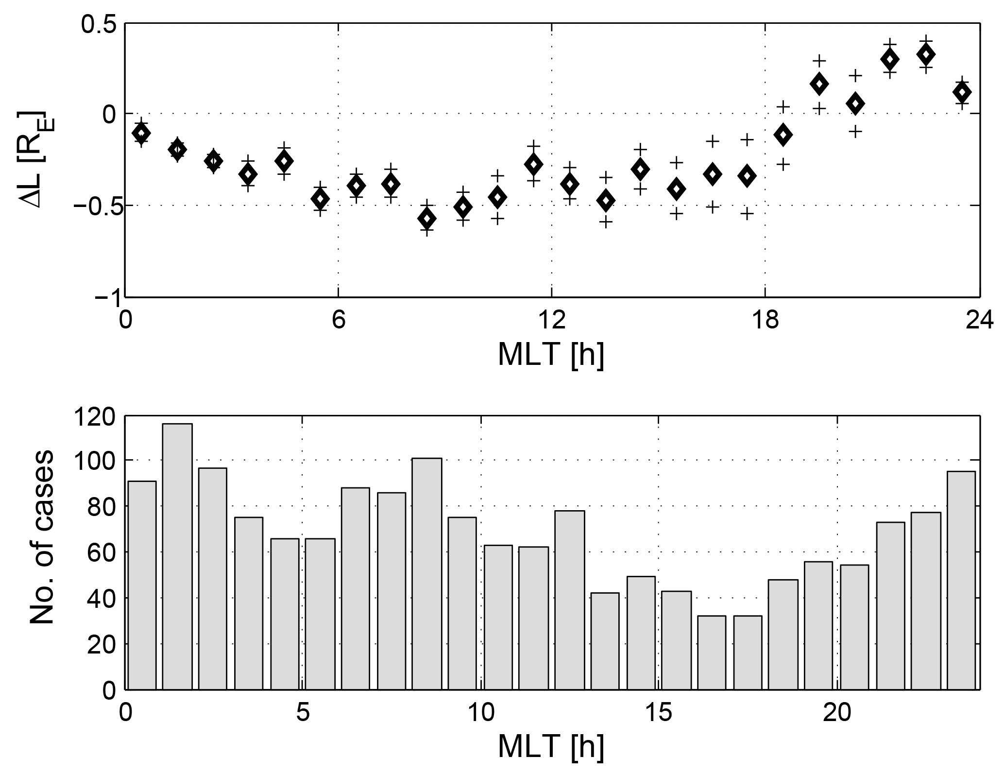
Figure 13Mean difference between VAP PP_N_e position and Swarm SSFAC index as a function of MLT.

Download

We also estimated the mean separation between the boundaries as a function of MLT from 1665 Swarm crossings (Fig. 13). SSFAC indices and simultaneous (UT difference is less than ±1 h) VAP PP_N_e positions were compared. The comparison revealed a clear bulge signature in the pre-midnight sector (19:00–01:00 MLT) peaking at 21:00–22:00 MLT. Elsewhere the SSFAC boundary is found typically poleward of the PP by ∼ 0.2 R. This result is very similar to the obtained differences between CHAMP and IMAGE observations. However, for individual cases the location of the boundaries can be very different. While the PP_N_e shape, due to its co-rotation with Earth and the localized erosion, is determined by the Kp evolution in the preceding days, the SSFAC index responds within a few hours simultaneously at all MLTs. This difference has important implications for the derivation of a future PP model that is based on SSFAC boundary detections.

From our results it is clear that the PP_N_e does not follow closely the SSFAC boundary. The shape of the latter corresponds more to an equatorial cut of a drift shell, and soft electrons may precipitate from this drift shell into the ionosphere. Precipitation enhances the conductance of the ionosphere, leading to increased current density. Indeed, Xiong and Lühr (2014) derived a model of the auroral oval boundaries from SSFAC signatures observed at LEO. Their equatorward boundary defined as the highest poleward gradient in log squared SSFAC density equatorward of the maximum is consistently poleward of our SSFAC boundary; since our fixed threshold is low, at 0.01 µA m⁻², the mean FAC density at their boundary is more than an order of magnitude higher. The PP typically maps to the sub-auroral ionosphere, where the conductance is smaller than in the auroral oval. Moving poleward from low latitudes, the first SSFACs appear just outside the PP_N_e. We believe that this is the reason why the SSFAC boundary is collocated with the night side PP_N_e under quiet conditions. Our plan for the future is to investigate the dynamic linkage among the elements of this complex system.

Swarm FAC data are available through the ESA Earth Online platform, after registration for an ESA Earth Observation Users' Single Sign On account https://earth.esa.int/web/guest/ umsso?orig_request=/web/guest/picommunity/myearthnet (ESA, 2018). VAP electron density data are openly available at the ftp site of the Space Environment Modeling Group at UCLA (ftp://rbm.epss.ucla.edu/ftpdisk1/NURD/) (UCLA, 2016). Geomagnetic indices (Kp, Dst, AE) and the solar wind data were retrieved through the NASA OMNIWeb space physics data facility at http://omniweb.gsfc.nasa.gov/ (GSFC, 2018).

The authors declare that they have no conflict of interest.

This article is part of the special issue “Dynamics and interaction of processes in the Earth and its space environment: the perspective from low Earth orbiting satellites and beyond”. It is not associated with a conference.