the Creative Commons Attribution 4.0 License.
the Creative Commons Attribution 4.0 License.
 | 03 Apr 2018
High-resolution vertical velocities and their power spectrum observed with the MAARSY radar – Part 1: frequency spectrum
Markus Rapp
Gunter Stober
Ralph Latteck
The Middle Atmosphere Alomar Radar System (MAARSY) installed at the island of Andøya has been run for continuous probing of atmospheric winds in the upper troposphere and lower stratosphere (UTLS) region. In the current study, we present high-resolution wind measurements during the period between 2010 and 2013 with MAARSY. The spectral analysis applying the Lomb–Scargle periodogram method has been carried out to determine the frequency spectra of vertical wind velocity. From a total of 522 days of observations, the statistics of the spectral slope have been derived and show a dependence on the background wind conditions. It is a general feature that the observed spectra of vertical velocity during active periods (with wind velocity > 10 m s−1) are much steeper than during quiet periods (with wind velocity < 10 m s−1). The distribution of spectral slopes is roughly symmetric with a maximum at −5/3 during active periods, whereas a very asymmetric distribution with a maximum at around −1 is observed during quiet periods. The slope profiles along altitudes reveal a significant height dependence for both conditions, i.e., the spectra become shallower with increasing altitudes in the upper troposphere and maintain roughly a constant slope in the lower stratosphere. With both wind conditions considered together the general spectra are obtained and their slopes are compared with the background horizontal winds. The comparisons show that the observed spectra become steeper with increasing wind velocities under quiet conditions, approach a spectral slope of −5/3 at a wind velocity of 10 m s−1 and then roughly maintain this slope (−5/3) for even stronger winds. Our findings show an overall agreement with previous studies; furthermore, they provide a more complete climatology of frequency spectra of vertical wind velocities under different wind conditions.
Keywords. Meteorology and atmospheric dynamics (turbulence; waves and tides)


Mesoscale motions in the atmosphere (a range of temporal scale from several minutes to about 2 days and spatial scale from several hundred meters to about 1000 km) are key to understand the interactions between atmospheric motions at large and small scales. The characteristics of wind and temperature fluctuations at different scales are typically described by means of their power spectra versus frequency and/or spatial scale. Measurements using different techniques, i.e., radiosondes, aircraft, and radars, have shown that power spectra of horizontal velocities as a function of frequency (or wavenumber) generally follow a (or ) power law (where f refers to frequency and k to wavenumber) (e.g., Gage, 1979; Basley and Carter, 1982; Larsen et al., 1986), although deviations from this slope have also been observed such that a −5/3 power law can not be assumed to be universal (e.g., Larsen et al., 1982). Even after three decades of study, the mechanisms producing the −5/3 spectrum in the mesoscale regime remain to be controversial (e.g., Gage, 1979; Gage and Nastrom, 1990; Larsen et al., 1982; Lilly, 1983; Vallis et al., 1997; Koshyk et al., 1999; Tung and Orlando, 2003, 2004; Smith, 2004; Lindborg, 2006; Brune and Becker, 2013; Callies et al., 2016; Bierdel et al., 2016, and many others). One of the explanations is that the mesoscale spectrum is the production of inertia-gravity waves (e.g., VanZandt, 1982; Dewan, 1997), which is similar to the classical Garrett–Munk spectrum found in the ocean (Garrett and Munk, 1975). Alternative explanations have also been proposed that this spectrum is due to a quasi-two-dimensional turbulent vortical flow (Gage, 1979; Lilly, 1983) or to stratified turbulence (Lindborg, 2006).
Vertical velocity of air motion contains key information on various dynamical processes in the lower and middle atmosphere like turbulence, gravity wave, and tidal motions. In order to understand the underlying mechanisms responsible for the atmospheric motions in the mesoscale range, the vertical velocity spectra should be further studied. So far, however, only a few studies have been carried out focusing on the frequency spectra of vertical velocities. The pioneer work using radar may go back to Röttger (1981) who analyzed the SOUSY-VHF-Radar observations. Ecklund et al. (1986) gave a preliminary climatology of the frequency spectra of vertical velocity derived by analyzing the data taken from radars at four widely separated geographical locations. Under quiet conditions with weak winds (< 10 m s−1), their spectra show a nearly constant slope close to 0 at periods larger than the Brunt–Vaisälä period τB, a bump (i.e., excess energy) at τB, and a rapid drop-off beyond τB. Under active conditions with strong winds, however, the spectra show slopes close to −5/3 with no localized maxima. Mean spectra averaged over both active and quiet periods approach a f−1 dependence. Based on the analysis of 15-day measurements with the SOUSY-VHF-Radar, Larsen et al. (1987) presented slopes close to −1 for the frequency spectra of vertical velocity in the lower troposphere, decreasing towards a slope near −1/2 around the tropopause and in the lower stratosphere. However, Muschinski et al. (2001) determined frequency spectra of vertical velocity from 72 h of observations with the SOUSY-VHF-Radar and presented the spectral drop-off beyond τB with slopes approaching −5/3 at moderate and strong winds and as steep values as −3 or −4 for weak winds. Although mean frequency spectra of horizontal velocities are fairly consistent with models, typically showing slopes with a constant value close to −5/3 with only slight amplitude variations (Basley and Carter, 1982; Basley and Garello, 1985; Fritts et al., 1990), the vertical velocity spectra are characterized by more variabilities in slopes, i.e., following a f2−p power law, where p is a constant ranging from 5/3 to 4 (VanZandt et al., 1991). Therefore, the underlying mechanisms as well as the climatology of the vertical velocity spectra are still important open issues for further investigation.
In this study, we apply the Lomb–Scargle periodogram method to determine the statistics of the power spectra of vertical velocity versus frequency (or period) using the Middle Atmosphere Alomar Radar System (MAARSY; see Latteck et al., 2010, 2012, for details on the radar system) and to study their correlation with the background wind fields. In Sect. 2, we describe the radar system of MAARSY including the experimental setup and the wind observations. In Sect. 3, the analysis method is outlined. The distribution of the derived spectral slopes and their dependence on the background wind fields are given and discussed in Sect. 4. Our conclusions are finally summarized in Sect. 5.
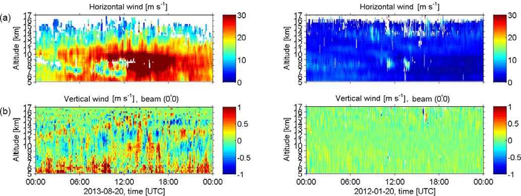
Figure 1Height–time intensity of wind measurements with MAARSY running a tropospheric experiment on 20 August 2013 (left panels) and 20 January 2012 (right panels). Upper panels are horizontal winds and lower panels are vertical winds.

Figure 2A climatology of horizontal wind velocities obtained by MAARSY. (a) Number densities of horizontal wind velocity in logarithmic scale and the white line indicates the mean profile of wind velocities along the altitudes; (b) distributions of wind velocity grouped into four height gates for every ∼ 3 km from ∼ 5 to 17 km.
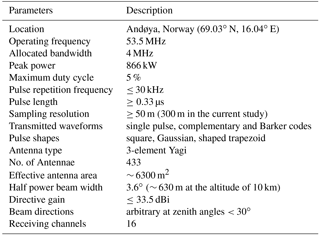
In the current study we analyzed measurements performed with the Middle Atmosphere Alomar Radar System (MAARSY) installed on the northern Norwegian island of Andøya (69.03∘ N, 16.04∘ E). The basic parameters of MAARSY relevant to our study are summarized in Table 1. A detailed technical description of MAARSY is given by Latteck et al. (2010, 2012).
MAARSY is able to perform multi-channel recording allowing for combining spaced antenna and Doppler measurements in the same experiment to investigate the atmospheric wind fields. In this work we apply the Doppler beam swinging (DBS) technique to estimate horizontal winds (both zonal and meridional) from five beams (one in the vertical direction and four at an off-zenith angle of 10∘ in orthogonal azimuths) with a temporal resolution of 5 min (e.g., Röttger and Larsen, 1990; Stober et al., 2012, 2013; Li et al., 2016). Note that the DBS method is able to determine a full three-dimensional wind vector including the vertical direction. However, it is well known that the vertical wind velocities derived from the DBS technique are biased due to the fitting procedure, i.e., averaging radial velocities on all five beams for 5 min leading to unexpected high-frequency peaks in their power spectra (not shown here). For the current study, we thus take the radial velocities along the vertical beam as vertical velocities.
Figure 1 shows two examples of wind measurements with MAARSY on 20 August 2013 and 20 January 2012. The blank areas in the upper panels are due to the averaging procedure for horizontal wind estimates with the DBS technique. The measurements on 20 August 2013 show much stronger horizontal winds, especially in the troposphere, and correspondingly stronger vertical wind fluctuations than on 20 January 2012.
From a total of 522 days of wind measurements with MAARSY, we present a climatology of horizontal wind velocity which is shown in Fig. 2. The number densities of wind values versus altitudes are shown in logarithmic scales (see the left panel of Fig. 2). Generally, horizontal winds are stronger in the upper troposphere than in the lower stratosphere. The mean altitude profile of horizontal winds indicated by the white line shows an increase along altitudes in the upper troposphere, i.e., from ∼ 5 km up to the tropopause height, which ranges between ∼ 9.2 and 10.5 km derived from temperature profiles taken from the ECMWF reanalysis data (Dee et al., 2011; not shown here) and a decrease along altitudes in the lower stratosphere. Following the analysis method by Parton et al. (2010), we group the wind velocities into four height gates of ∼ 3 km width and the probability densities are shown in the right panel of Fig. 2. The horizontal wind velocities follow a very asymmetric distribution with a peak lying within the range of 0–10 m s−1 and a long tail towards values as large as ∼ 80 m s−1. For the altitude gate between 8.0 and 11.0 km, the horizontal wind velocities reveal a clear indication of a bimodal structure with a second peak at a value of ∼ 16 m s−1. Further, the probability densities of wind velocity both show a “shoulder” with values between ∼ 10 and 20 m s−1 for the altitude gates of 5.0–8.0 km and of 11.0–14.0 km. A possible explanation for this bimodal structure is that the wind velocity distribution is sensitive to the effect of weather systems passing over such that a separate analysis of cyclonic and non-cyclonic periods should be considered (Parton et al., 2010).
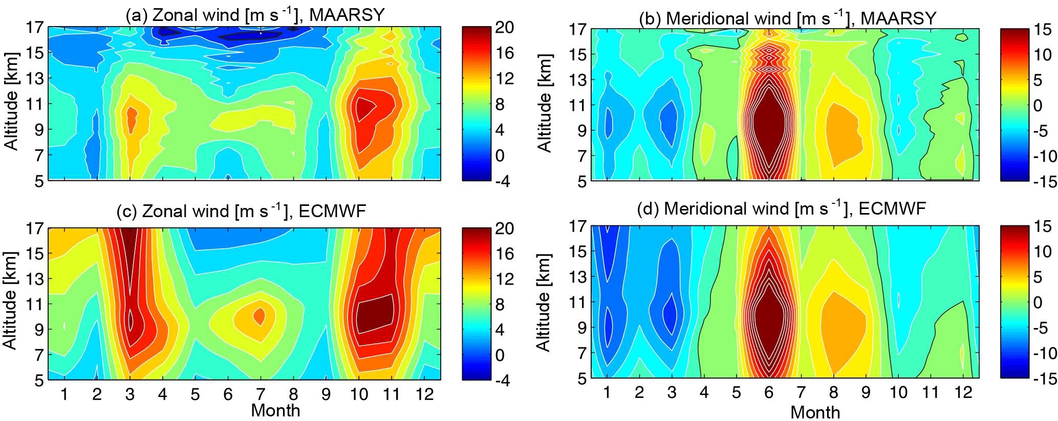
Figure 3Seasonal variations in monthly-mean wind velocity for a composite year derived from MAARSY (a, b) and the ECMWF reanalysis data (c, d) based on identical sampling between both zonal winds in the left panels and meridional winds in the right panels. The zero-velocity contours are indicated in black and the white contours in a step of 2 m s−1. Positive values are for eastward and northward winds.
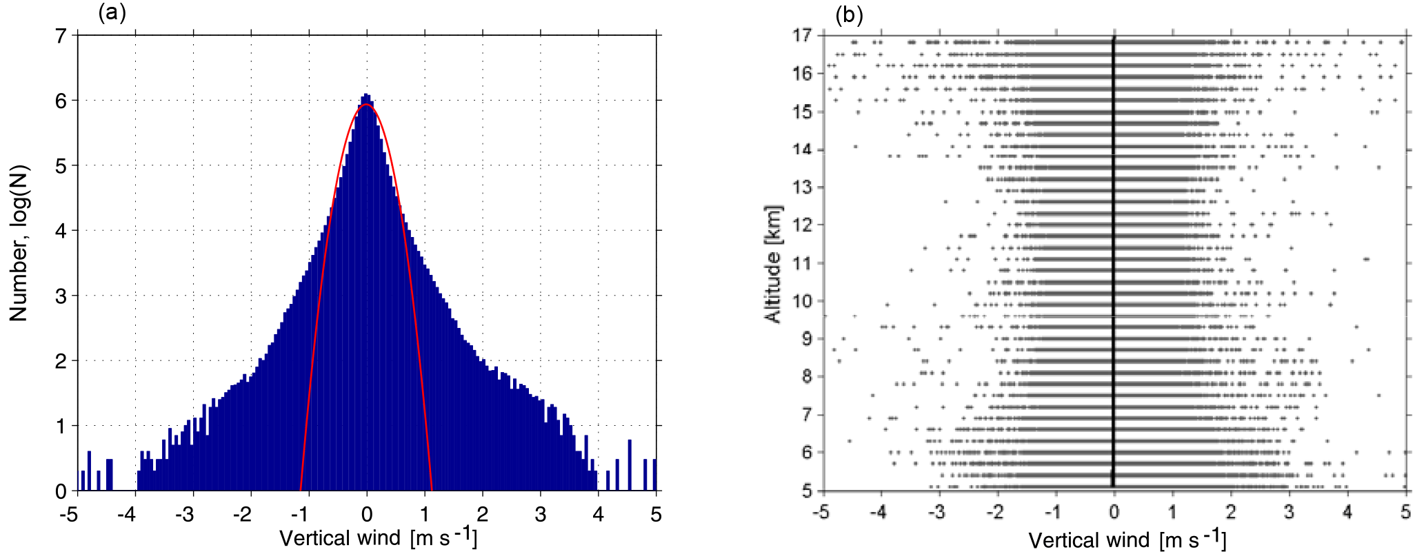
Figure 4(a) Histogram of number densities of vertical wind velocity in logarithmic scales with the fitting line by a Gaussian function indicated in red; (b) scatter plot of vertical wind velocities along the altitudes with the mean profile indicated with a black solid line.
Monthly-mean zonal and meridional winds recorded with MAARSY and taken from the ECMWF reanalysis data based on identical sampling (i.e., the ECMWF winds are only sampled for analysis during the periods when radar measurements are available.) between 5 and 17 km are reproduced for a composite year in Fig. 3. The comparison between the radar measurements and the model shows a quite similar pattern of a significant seasonal variation. In the left panels, the main features of the data are a dominant eastward zonal wind in the UTLS regions and the strongest wind occurring near the tropopause height covering the polar jet stream. Seasonal variation in zonal winds shows the strongest zonal winds in March and October, especially from the ECMWF winds, and a secondary peak of zonal winds appears in summer just below the tropopause. The minima of zonal wind appear between ∼ 15 and 17 km in summer. Monthly-mean meridional winds also show a prominent seasonal variation, namely poleward (northward) winds occurring from April to October and equatorward (southward) winds in the other months. The maxima of the meridional wind appear in June and August for the poleward winds and in January and March for the equatorward winds. Meridional winds were found to be as large as 50 m s−1 in June. Note, however, that the statistics in June are very poor, i.e., only 4 days with radar measurements were possible in 2013. Furthermore, the ECMWF reanalysis data give slightly stronger winds (both zonal and meridional winds) compared to the radar measurement.
It is mentioned above that the vertical wind velocities in this work are taken from the radial velocities along the vertical beam. The distribution of vertical velocities is shown in Fig. 4. The vertical velocities roughly follow a symmetric distribution with a peak around zero (see the left panel of Fig. 4). The vertical velocities vary within a range between −4 and 4 m s−1 (with the probability density less than 1/105 of the maximum). A Gaussian distribution function is regressed to the histogram of vertical velocity and the fitting line is overlayed in red. We note that the vertical velocities do not follow a Gaussian distribution, but an intermittent distribution with a tail extending to higher velocities which is typical for a turbulent medium (e.g., Schertzer and Lovejoy, 1985; Jiménez, 2007; Neelin et al., 2010). Please note, however, that intermittency is also one of the properties of gravity waves (e.g., Hertzog et al., 2012). It hence cannot be precluded that the gravity waves have influence on the resulting non-Gaussian distribution of vertical velocities. The right panel of Fig. 4 shows all obtained vertical wind velocities with the mean altitude profile with a solid line. The vertical velocities at the altitude range of 9–11 km (covering the tropopause height) possess a narrower range compared to the upper and lower altitudes, i.e., smaller vertical velocity variance near the tropopause height. The mean profile shows values ranging between ∼ −3 and −1 cm s−1. We should mention here, however, that these values must be taken with care since systematic biases arise when computing long-term mean vertical winds from radar measurements, which can be caused by many complications such as locations and instrumental impreciseness (see the review by Hocking, 2011). The downward bias of the observed vertical velocities have long been noticed and are very common. Previous studies for the explanation reported that vertical velocities are influenced by gravity waves with upward energy propagation as well as by the condition of Kelvin–Helmholtz instabilities appearing above and below the jet streams (strong horizontal winds; e.g., Nastrom and VanZandt, 1994; Hoppe and Fritts, 1995; Muschinski, 1996). However, the mechanism of how gravity waves and/or Kelvin–Helmholtz instabilities affect the measurements of vertical wind is beyond the scope of this current study.
Time series of wind measurements obtained by radar are often characterized by incomplete or uneven sampling due to the system operation and removal of outliers. Spectral analysis using fast Fourier transform (FFT) hence requires some degree of interpolation to fill in gaps, which may introduce uncontrolled frequency components and complicate the analysis. A number of alternatives have been put forward to handle the unevenly sampled data. The Lomb–Scargle periodogram developed by Lomb (1976) and Scargle (1982) is a widely used method, which estimates a power spectrum at each frequency or period based on a least-squares fit of sinusoids (Press et al., 2007).
In this study, we first subtract the mean from the time series of vertical wind velocity and subsequently perform spectral analysis of the residuals to calculate the Lomb–Scargle periodogram of vertical velocity based on the following equation (Press et al., 2007),
where ω is the angular frequency and Xj=X(tj), is the value of the physical quantity (here vertical velocity) measured in time tj; and σ2 are the mean and variance in vertical velocities calculated based on the usual formulas: and . Here τ is a time delay defined by
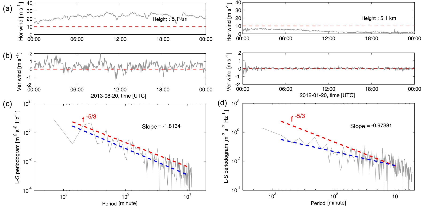
Figure 5Power spectra of vertical wind velocity versus period (or frequency) using Lomb–Scargle periodogram during active (c) and quiet periods (d). Horizontal and vertical winds are plotted in (a) and (b), respectively. The lines of horizonal winds = 10 m s−1 and vertical winds = 0 m s−1 are also shown in red as reference. Note that the frequency cutoffs depend on the time resolution of the analyzed data set (2–5 min for the current study).
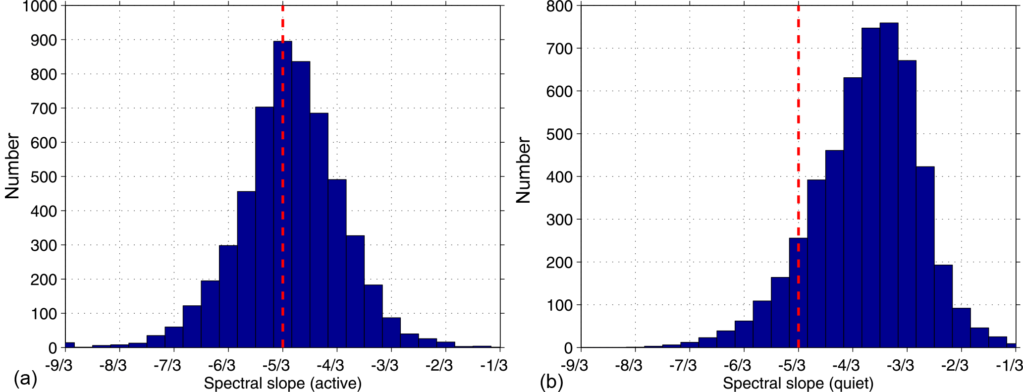
Figure 6Histograms of spectra of vertical wind velocity during active (a) and quiet periods (b). The theoretical −5/3 spectral slope is indicated by the red dashed line.
Two examples of Lomb–Scargle periodograms of vertical velocities under different conditions of background winds are shown in Fig. 5. Here we define quiet conditions as background winds with velocities < 10 m s−1 over a 24 h period and active conditions as velocities > 10 m s−1 following the wind criterion by Ecklund et al. (1986). The Lomb–Scargle periodograms of vertical velocity under active and quiet wind conditions are shown in the lower panels of Fig. 5 (active conditions in the left and quiet conditions in the right). Typically, the Brunt–Väisälä period τB is about 10 min in the troposphere and about 5 min in the stratosphere and the inertial period is ∼ 18 h (i.e., ∼ 1000 min). We hence regress the logarithm of the spectrum for periods between 1000 and 10 min. The fitting lines are indicated by the blue dashed lines. The slopes of the fitting line are indicated in the insert. We also indicate a theoretical spectral slope of −5/3 in red for reference. The comparisons under different wind conditions show that the spectral slope approaches the law under active conditions and becomes shallower (roughly f−1) under quiet conditions. The vertical velocity spectra during the quiet period show a rough peak near the period slightly larger than 10 min (τB). Such peaks are more apparent at the higher altitudes (∼ 5 min in the stratosphere, not shown here) and are assumed to be physically real due to propagating gravity waves at τB (Röttger and Ierkic, 1985). During the active period, however, there are no clear peaks at τB, rather the spectrum follows the same power law beyond τB to the minimum period. Further, the comparison between both spectra indicate no clear cutoff beyond τB observed under active conditions. This is consistent with the fact that the frequency spectra of vertical velocity are highly sensitive to Doppler-shifting effects (Scheffler and Liu, 1986; Fritts and VanZandt, 1987).
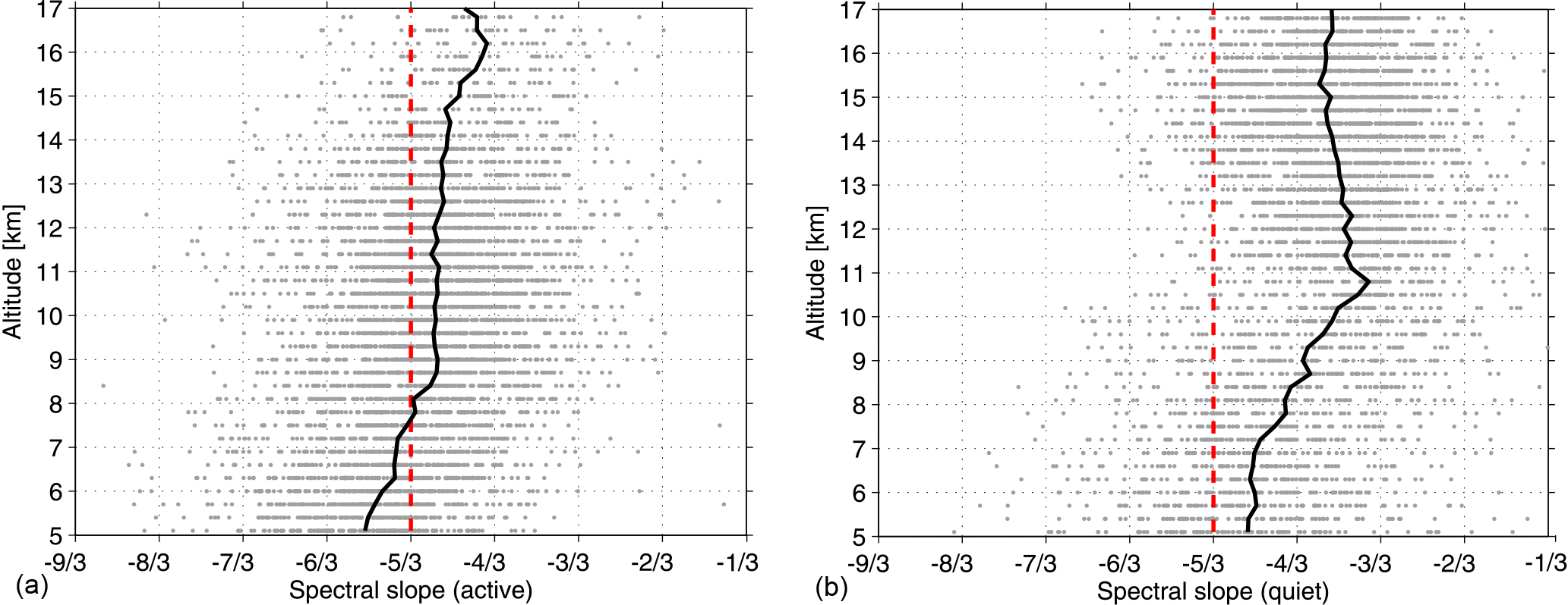
Figure 7Scatter plots of spectra of vertical wind velocity during active (a) and quiet periods (b). The black lines indicate the mean profiles of the spectral slope along the altitudes. The theoretical −5/3 spectral slope is indicated by the red dashed line.

Figure 8Dependence of the general spectral slope of vertical wind velocity on the background wind fields. The black dashed line indicates the horizontal wind = 10 m s−1.
The overall results of performing this analysis on the available data set of 522 days are presented in Fig. 6. Note that we here define active (quiet) conditions by the requirement that 90 % of wind velocities over a 24 h period are larger (smaller) than 10 m s−1. Our choice of this definition was revealed to be optimum to avoid false removal of any active (or quiet) conditions because of the fact that there are substantial variabilities in the wind measurements due to waves and/or system noise. This definition also indicates that the wind observations with gaps larger than 10 % of a 24 h period will be neglected. Figure 6 reveals that the derived spectral slopes under active conditions (left panel) follow a roughly symmetric distribution around a mean of ∼ −5/3 with minimum and maximum values between −8/3 and −2/3. This is consistent with theory and previous studies (e.g., Scheffler and Liu, 1985; Ecklund et al., 1985; Gage et al., 1986). Under quiet conditions (right panel), however, the spectral slopes follow a very asymmetric distribution with a long tail extending towards smaller values with a maximum at around −10/9, which is close to −1. Furthermore, we also present a plot of all individual spectral slopes along altitudes with the altitude-mean profiles indicated by black solid lines in Fig. 7. Again the theoretical spectral slopes of are overlayed in red for reference. Figure 7 clearly shows that the number densities are much larger under active conditions at lower altitudes (below ∼ 11 km) than under quiet conditions at upper altitudes (above ∼ 12 km), which is consistent with the distribution of horizontal wind velocities shown in Fig. 2. The spectral slopes for both conditions first reveal a decrease (i.e., spectra become shallower) with increasing altitude and then maintain at a roughly constant value. These “break points” are at ∼ 9 km for active conditions and ∼ 10.5 km for quiet conditions, which are close to the tropopause heights. A similar height dependence of spectral slopes was also reported by previous studies (e.g., Kuo et al., 1985; Larsen et al., 1987). When active and quiet periods are considered together (i.e., the whole data set is analyzed despite the background wind conditions), the so-called “general” spectra of vertical velocity are derived and reveal intermediate slopes compared with those under active or quiet conditions. In Fig. 8, we present the general spectra of vertical wind derived from the whole data set versus the corresponding horizontal winds. The dependence of the spectral slopes on the background horizontal winds shows clear different variations separated at a wind threshold of ∼ 10 m s−1. During quiet periods (wind velocity < 10 m s−1), the observed spectra of vertical wind velocity show that their slopes (absolute values) are roughly positively correlated with the background wind velocities. More precisely, with increasing wind velocities, the spectral slopes increase starting from −1/3 and approach the −5/3 spectral slope which has been observed for the spectra of horizontal wind velocities. During active periods, however, the spectral slopes maintain a nearly constant value of −5/3, especially with stronger winds (e.g., velocities > 15 m s−1), although their distribution falls within a range between ∼ −1 and −7/3.
In this paper, we presented tropospheric and lower stratospheric wind measurements using the MAARSY MST radar (Mesosphere–Stratosphere–Troposphere). From a total of 522 days of observations, we presented the distribution of horizontal winds. The wind velocities are stronger in the upper troposphere than in the lower stratosphere. Further, the mean altitude profile shows that the wind velocities increase with altitude in the upper troposphere, reach the largest values close to the tropopause height and then decrease with altitude in the lower stratosphere. The wind velocities have been grouped into different height gates for every ∼ 3 km and the probability densities follow a very asymmetric distribution with peaks lying within the range of ∼ 0–10 m s−1 and a long tail extending to ∼ 80 m s−1. The seasonal variation in meridional and zonal winds have been derived and compared with the results from the ECMWF reanalysis data based on identical sampling. There is a dominant eastward zonal wind in the UTLS region and the strongest winds occurred within the altitudes close to the tropopause height (∼ 9.2–10.5 km). The meridional winds show a poleward direction from April to October and equatorward in the other months. Vertical winds are taken from the radial velocities along the vertical beam. Their distribution cannot be characterized by a Gaussian function but an intermittent distribution which is typical for a turbulent medium. The mean altitude profiles of vertical velocity show slightly negative values (< −3 cm s−1; i.e., downward bias), which is commonly considered as a bias due to either wave or Kelvin–Helmholtz dynamics.
We calculated the frequency spectra of vertical wind velocities by performing the Lomb–Scargle periodogram method for both active and quiet wind conditions, following the criteria of wind conditions by Ecklund et al. (1986). The statistics of the observed spectra of vertical velocity for both conditions are derived from the analysis of 522-day radar observations. The spectral slopes follow a roughly symmetric distribution with a maximum probability at −5/3 during active periods, whereas a very asymmetric distribution with a maximum probability at around −1 is observed during quiet periods. The scatter plot of the slopes with the mean altitude profile for both conditions reveal a decrease (i.e., the spectra become shallower) with increasing altitudes in the troposphere and then maintain a roughly constant value in the lower stratosphere (even slightly decreasing with increasing altitudes for quiet conditions). Taking all data together, the general spectra of vertical wind velocity reveal intermediate slopes compared with the spectra under active or quiet conditions. Furthermore, we compared the general spectral slopes of vertical velocity with the background horizontal winds and found that the dependence of the spectra of vertical winds on the background horizontal winds reveal different properties under different wind conditions. During quiet periods, the spectral slopes of vertical winds starting at around −1/3 show an increase with increasing horizontal wind velocities and approach −5/3 at a wind threshold of ∼ 10 m s−1. During active periods, however, the spectral slopes maintain a nearly constant value of −5/3 which matches the slopes of the horizontal wind spectra. These results provide a more complete climatology of frequency spectra of vertical wind velocities under different wind conditions from high-resolution wind measurements with MAARSY compared with previous studies.
The data sets with the MAARSY radar used in this study are stored in the Leibniz-Institut für Atmosphärenphysik (IAP) repository and are available upon request to the author (contact email: chau@iap-kborn.de).
The authors declare that they have no conflict of interest.
The authors would like to thank Jorge L. Chau for support of MAARSY data
handling. Qiang Li and Markus Rapp acknowledge support by the German Ministry for
Education and Research (BMBF) in the scope of the ROMIC-GWLCYCLE Project.
Support for Gunter Stober and Ralph Latteck was provided by the BMBF ROMIC-METROSI
Project – 01LG1218A.
The article processing charges for this open-access
publication were covered by a Research
Centre of the Helmholtz Association.
The topical editor, Petr Pisoft, thanks two anonymous referees for help in evaluating this paper.
Basley, B. B. and Carter, D. A.: The spectrum of atmospheric velocity fluctuations at 8 km and 86 km, Geophys. Res. Lett., 9, 465–468, 1982. a, b
Basley, B. B. and Garello, R.: The kinetic energy density in the troposphere, stratosphere adn mesosphere: A preliminary study using the Poker Flat radar in Alaska, Radio Sci., 20, 1355–1362, 1985. a
Bierdel, L., Snyder, C., Park, S.-H., and Skamarock, W. C.: Accuracy of rotational and divergent kinetic energy spectra diagnosed from flight-track winds, J. Atmos. Sci., 73, 3273–3286, https://doi.org/10.1175/JAS-D-16-0040.1, 2016. a
Brune, S. and Becker, E.: Indication of stratified turbulence in a Mechanistic GCM, J. Atmos. Sci., 70, 231–247, https://doi.org/10.1175/JAS-D-12-025.1, 2013. a
Callies, J., Bühler, O., and Ferrari, R.: The dynamics of mesoscale winds in the upper troposphere and lower stratosphere, J. Atmos. Sci., 73, 4853–4872, https://doi.org/10.1175/JAS-D-16-0108.1, 2016. a
Dee, D. P., Uppala, S. M., Simmons, A. J., Berrisford, P., Poli, P., Kobayashi, S., Andrae, U., Balmaseda, M. A., Balsamo, G., Bauer, P., Bechtold, P., Beljaars, A. C. M., van de Berg, L., Bidlot, J., Bormann, N., Delsol, C., Dragani, R., Fuentes, M., Geer, A. J., Haimberger, L., Healy, S. B., Hersbach, H., Hólm, E. V., Isaksen, L., Kållberg, P., Köhler, M., Matricardi, M., McNally, A. P., Monge-Sanz, B. M., Morcrette, J.-J., Park, B.-K., Peubey, C., de Rosnay, P., Tavolato, C., Thépaut, J.-N., and Vitart, F.: The ERA-Interim reanalysis: configuration and performance of the data assimilation system, Q. J. Roy. Meteor. Soc., 137, 553–597, https://doi.org/10.1002/qj.828, 2011. a
Dewan, E.: Saturated-cascade similitude theory of gravity wave spectra, J. Geophys. Res., 102, 29799–29817, 1997. a
Ecklund, W. L., Balsley, B. B., Carter, D. A., Riddle, A. C., Crochet, M., and Garello, R.: Observations of vertical motions in the troposphere and lower stratosphere using three closely spaced ST radars, Radio Sci., 20, 1196–1206, 1985. a
Ecklund, W. L., Gage, K. S., Nastrom, G. D., and Balsley, B. B.: A preliminary climatology of the spectrum of vertical velocity observed by clear-air Doppler radar, J. Climate Appl. Meteor., 25, 885–892, 1986. a, b, c
Fritts, D. C. and VanZandt, T. E.: Effects of Doppler shifting on the frequency spectra of atmospheric Gravity waves, J. Geophys. Res., 92, 9723–9732, 1987. a
Fritts, D. C., Tsuda, T., VanZandt, T. E., Smith, S., Sato, T., Fukao, S., and Kato, S.: Studies of velocity fluctuations in the lower atmosphere using the MU radar. Part II: Momentum fluxes and energy densities, J. Atmos. Sci., 47, 51–66, 1990. a
Gage, K. S.: Evidence for a law inertial range in mesoscale two-dimensional turbulence, J. Atmos. Sci., 36, 1950–1954, 1979. a, b, c
Gage, K. S. and Nastrom, G. D.: A simple model for the enhanced frequency spectrum of vertical velocity based on tilting of atmospheric layers by lee waves, Radio Sci., 25, 1049–1056, 1990. a
Gage, K. S., Balsley, B. B., and Garello, R.: Comparisons of horizontal and vertical velocity spectra in the mesosphere, stratosphere and troposphere: Observations and theory, Geophys. Res. Lett., 13, 1125–1128, 1986. a
Garrett, C. and Munk, W.: Space-time scales of internal waves: A progress report, J. Geophys. Res., 80, 291–297, 1975. a
Hertzog, A., Alexander, M. J., and Plougonven, R.: On the intermittency of gravity wave momentum flux in the stratosphere, J. Atmos. Sci., 69, 3433–3448, https://doi.org/10.1175/JAS-D-12-09.1, 2012. a
Hocking, W. K.: A review of Mesosphere-Stratosphere-Troposphere (MST) radar developments and studies, circa 1997–2008, J. Atmos. Sol.-Terr. Phy., 73, 848–882, 2011. a
Hoppe, U.-P. and Fritts, D. C.: On the downward bias in vertical velocity measurements by VHF radars, Geophys. Res. Lett., 22, 619–622, https://doi.org/10.1029/95GL00165, 1995. a
Jiménez, J.: Intermittency in turbulence, in: Proc. 15th “Aha Huliko” a Winter Workshop, Extreme Events, 81–90, 2007. a
Koshyk, J. N., Hamilton, K., and Mahlmann, J. D.: Simulation of the mesoscale spectral regime in the GFDL SKYHI general circulation model, Geophys. Res. Lett., 26, 843–846, 1999. a
Kuo, F.-S., Shen, H.-W., Fu, I.-J., Chao, J.-K., Röttger, J., and Liu, C.-H.: Altitude dependence of vertical velocity spectra observed by VHF radar, Radio Sci., 20, 1349–1354, 1985. a
Larsen, M. F., Kelley, M. C., and Gage, K. S.: Turbulence spectra in the upper troposphere and lower stratosphere at periods between 2 hours and 40 days, J. Atmos. Sci., 39, 1035–1041, 1982. a, b
Larsen, M. F., Woodman, R. F., Sato, T., and Davis, M. K.: Power spectra of oblique velocities in the troposphere and lower stratosphere observed at Arecibo, Puerto Rico, J. Atmos. Sci., 43, 2230–2240, 1986. a
Larsen, M. F., Röttger, J., and Holden, D. N.: Direct measurements of vertical-velocity power spectra with the SOUSY-VHF-Radar wind profiler system, J. Atmos. Sci., 44, 3442–3448, 1987. a, b
Latteck, R., Singer, W., Rapp, M., and Renkwitz, T.: MAARSY – the new MST radar on Andøya/Norway, Adv. Radio Sci., 8, 219–224, https://doi.org/10.5194/ars-8-219-2010, 2010. a, b
Latteck, R., Singer, W., Rapp, M., Vandepeer, B., Renkwitz, T., Zecha, M., and Stober, G.: MAARSY: The new MST radar on Andøya – System description and first results, Radio Sci., 47, RS1006, https://doi.org/10.1029/2011RS004775, 2012. a, b
Li, Q., Rapp, M., Schrön, A., Schneider, A., and Stober, G.: Derivation of turbulent energy dissipation rate with the Middle Atmosphere Alomar Radar System (MAARSY) and radiosondes at Andøya, Norway, Ann. Geophys., 34, 1209–1229, https://doi.org/10.5194/angeo-34-1209-2016, 2016. a
Lilly, D. K.: Stratified turbulence and the mesoscale variability of the atmosphere, J. Atmos. Sci., 40, 749–761, 1983. a, b
Lindborg, E.: The effect of rotation on the mesoscale energy cascade in the free atmosphere, Geophys. Res. Lett., 32, L01809, https://doi.org/10.1029/2004GL021319, 2005. a, b
Lomb, N. R.: Least-squares frequency analysis of unequally spaced data, Astrophys. Space Sci., 39, 1841–1854, 1976. a
Muschinski, A.: Possible effect of Kelvin-Helmholtz Instability on VHF radar observations of the mean vertical wind, J. Appl. Meteor., 35, 2210–2217, 1996. a
Muschinski, A., Chilson, P. B., Palmer, R. D., Hooper, D. A., Schmidt, G., and Steinhagen, H.: Boundary-layer convection and diurnal variation of vertical-velocity characteristics in the free troposphere, Q. J. Roy. Meteor. Soc., 127, 423–443, 2001. a
Nastrom, G. D. and VanZandt, T. E.: Mean vertical motions seen by radar wind profilers, J. Appl. Meteor., 33, 984–995, 1994. a
Neelin, J. D., Lintner, B. R., Tian, B., Li, Q., Zhang, L., Patra, P. K., Chahine, M. T., and Stechmann, S. N.: Long tails in deep columns of natural and anthropogenic tropospheric tracers, Geophys. Res. Lett., 37, L05804, https://doi.org/10.1029/2009GL041726, 2010. a
Parton, G., Dore, A., and Vaughan, G.: A climatology of mid-tropospheric mesoscale strong wind events as observed by the MST radar, Aberystwyth, Meteorol. Appl., 17, 340–354, 2010. a, b
Press, W. H., Teukolsky, S. A., Vetterling, W. T., and Flannery, B. P.: Numerical recipes (3rd edition): the art of scientific computing, Cambridge University Press, NY, USA, 2007. a, b
Röttger, J.: Wind variability in the stratosphere deduced from spaced antenna VHF radar measurements, Preprints, 20th Conference on Radar Meteorology, AMS, 30 November–3 December 1981, Boston, USA, 1981, 22–29, 1981. a
Röttger, J. and Ierkic, H. M.: Postset beam steering and interferometer applications of VHF radars to study wind, waves and turbulence in lower and middle atmosphere, Radio Sci., 20, 1461–1480, 1985. a
Röttger, J. and Larsen, M. F.: UHF/VHF radar techniques for atmospheric research and wind profiler applications, Radar in Meteorology, D. Atlas, Ed., Amer. Meteor. Soc., 806 pp., 1990. a
Scargle, J. D.: Studies in astronomical time series analysis. II. Statistical aspects of spectral analysis of unequally spaced data, Astrophys. J., 302, 757–763, 1982. a
Scheffler, A. O. and Liu, C. H.: Observation of gravity wave spectra in the atmosphere using MST radars, Radio Sci., 20, 1309–1322, 1985. a
Scheffler, A. O. and Liu, C. H.: The effects of Doppler shift on gravity waves spectra observed by MST radar, J. Atmos. Terr. Phys., 48, 1225–1231, 1986. a
Schertzer, D. and Lovejoy, S.: The dimension and intermittency of atmospheric dynamics, in: Turbulent Shear Flows 4, edited by: Launder, B., 7–33, 1985. a
Smith, K. S.: Comments on “The k−3 and energy spectrum of atmospheric turbulence: Quasigeostrophic two level model simulation”, J. Atmos. Sci., 61, 937–942, 2004.. a
Stober, G., Latteck, R., Rapp, M., Singer, W., and Zecha, M.: MAARSY – the new MST radar on Andøya: first results of spaced antenna and Doppler measurements of atmospheric winds in the troposphere and mesosphere using a partial array, Adv. Radio Sci., 10, 291–298, https://doi.org/10.5194/ars-10-291-2012, 2012. a
Stober, G., Sommer, S., Rapp, M., and Latteck, R.: Investigation of gravity waves using horizontally resolved radial velocity measurements, Atmos. Meas. Tech., 6, 2893–2905, https://doi.org/10.5194/amt-6-2893-2013, 2013. a
Tung, K. K. and Orlando, W. W.: The k−3 and energy spectrum of atmospheric turbulence: Quasigeostrophic two level model simulation, J. Atmos. Sci., 60, 824–835, 2003. a
Tung, K. K. and Orlando, W. W.: “The k−3 and energy spectrum of atmospheric turbulence: Quasigeostrophic two level model simulation” – Reply, J. Atmos. Sci., 61, 943–948, 2004. a
Vallis, G. K., Shutts, G. J., and Gray, M. E. B.: Balanced mesoscale motion and stratified turbulence forced by convection, Q. J. Roy. Meteor. Soc., 123, 1621–1652, 1997. a
VanZandt, T. E.: A universal spectrum of buoyancy waves in the atmosphere, Geophys. Res. Lett., 9, 575–578, 1982. a
VanZandt, T. E., Nastrom, G. D., and Green, J. L.: Frequency spectra of vertical velocity from Flatland VHF radar data, J. Geophys. Res., 96, 2845–2855, 1991. a