the Creative Commons Attribution 4.0 License.
the Creative Commons Attribution 4.0 License.
 | 03 Apr 2018
New results on the mid-latitude midnight temperature maximum
Rafael L. A. Mesquita
John W. Meriwether
Jonathan J. Makela
Daniel J. Fisher
Brian J. Harding
Samuel C. Sanders
Fasil Tesema
Aaron J. Ridley
Fabry–Perot interferometer (FPI) measurements of thermospheric temperatures and winds show the detection and successful determination of the latitudinal distribution of the midnight temperature maximum (MTM) in the continental mid-eastern United States. These results were obtained through the operation of the five FPI observatories in the North American Thermosphere Ionosphere Observing Network (NATION) located at the Pisgah Astronomic Research Institute (PAR) (35.2∘ N, 82.8∘ W), Virginia Tech (VTI) (37.2∘ N, 80.4∘ W), Eastern Kentucky University (EKU) (37.8∘ N, 84.3∘ W), Urbana-Champaign (UAO) (40.2∘ N, 88.2∘ W), and Ann Arbor (ANN) (42.3∘ N, 83.8∘ W). A new approach for analyzing the MTM phenomenon is developed, which features the combination of a method of harmonic thermal background removal followed by a 2-D inversion algorithm to generate sequential 2-D temperature residual maps at 30 min intervals. The simultaneous study of the temperature data from these FPI stations represents a novel analysis of the MTM and its large-scale latitudinal and longitudinal structure. The major finding in examining these maps is the frequent detection of a secondary MTM peak occurring during the early evening hours, nearly 4.5 h prior to the timing of the primary MTM peak that generally appears after midnight. The analysis of these observations shows a strong night-to-night variability for this double-peaked MTM structure. A statistical study of the behavior of the MTM events was carried out to determine the extent of this variability with regard to the seasonal and latitudinal dependence. The results show the presence of the MTM peak(s) in 106 out of the 472 determinable nights (when the MTM presence, or lack thereof, can be determined with certainty in the data set) selected for analysis (22 %) out of the total of 846 nights available. The MTM feature is seen to appear slightly more often during the summer (27 %), followed by fall (22 %), winter (20 %), and spring (18 %). Also seen is a northwestward propagation of the MTM signature with a latitude-dependent amplitude. This behavior suggests either a latitudinal dependence of thermosphere tidal dissipation or a night-to-night variation of the composition of the higher-order tidal modes that contribute to the production of the MTM peak at mid-latitudes. Also presented in this paper is the perturbation on the divergence of the wind fields, which is associated with the passage of each MTM peak analyzed with the 2-D interpolation.
Keywords. Ionosphere (mid-latitude ionosphere)


The Earth's atmosphere is heated during the day by the absorption of solar energy and cooled at night by emission of thermal radiation energy to space. However, in the thermosphere there is seen quite often, near midnight, a temperature peak with an amplitude of up to 200 K. This phenomenon is called the midnight temperature maximum (MTM). This interesting nighttime phenomenon was first reported in the 1960s in ground-based optical, radar, and in situ measurements (Greenspan, 1966; Nelson and Cogger, 1971; Behnke and Harper, 1973; Spencer et al., 1979). Also associated with this temperature peak is a density enhancement called the midnight density maximum that has been detected with drag balance instruments on board the San Marco III and V satellites (Arduini et al., 1992, 1997; Arduini et al., 1993). These previous studies of the MTM phenomenon were carried out with observations within the 20∘ latitude range of the Equator. The present paper is unique as it presents results for the mid-latitude range between 30 and 45∘ latitude.
As discussed in the analysis of the Jicamarca nighttime radar measurements of electron temperatures, Bamgboye and McClure (1982) suggested the MTM peak resulted from the upward propagation of atmospheric tidal waves and is associated with a pressure/temperature bulge near midnight. Their work confirmed the equatorial MTM behavior described earlier by Herrero and Spencer (1982), which was based on a statistical analysis of the observations from the Neutral Atmosphere Temperature Experiment (NATE) mass spectrometer experiment on board of the Atmospheric Explorer-E (AE) satellite. These results showed a latitudinal distribution for the MTM that accounted for the seasonal variability in its peak amplitude within the latitude range covered by the AE satellite. Their findings show that the MTM is formed at the geographic Equator and propagates poleward and westward in both hemispheres. Regarding its seasonality, Herrero and Spencer (1982) noted the dominance of the MTM feature in the summer hemisphere, with the temperature maximum occurring earlier in local time and with higher amplitude when compared with the MTM behavior in the winter hemisphere.
The modeling work discussed by Mayr et al. (1979) concluded that the MTM is the result of a nonlinear interaction of the diurnal, semi-diurnal, and other higher-order tides. Colerico et al. (2006) reported on the sensitive influence of the terdiurnal as well as higher-order tidal modes that enhance the MTM peak amplitude. They suggested that the superposition of these higher-order tidal modes has a latitudinal distribution in such a way that the MTM amplitude would also be variable within a given latitude span. Determining this latitudinal variation of the MTM amplitude would help improve our understanding of how the overlap of these tidal modes at mid-latitudes may vary with latitude due to the individual latitudinal dependence of each tidal mode contributing to the overall tidal forcing from below. It is also possible that the contribution of a non-migrating tidal wave if significant may also vary with latitude.
The MTM latitudinal structure was recently modeled by Akmaev et al. (2009) to be a wake-wave shaped disturbance in temperature with a phase lag relative to the latitude; i.e., the timing of the MTM peak occurs later in the evening at higher latitudes. Their study confirms the MTM as being a result of the thermal part of the constructive interference between the upward propagating and in situ diurnal, semi-diurnal, and other higher-order migrating tidal modes (Akmaev et al., 2009; Akmaev, 2011). Among these important findings, Akmaev et al. (2009) found evidence for a weak secondary maximum in their Whole Atmosphere Model (WAM) occurring earlier in the evening. This result agrees with the detection of a secondary MTM peak that was reported by Faivre et al. (2006) from observations in the Peruvian sector. For the remainder of our paper, the terms “secondary” and “primary” refer to the earlier and later MTM peaks, respectively.
Colerico and Mendillo (2002) presented data showing the relationship between the MTM and the midnight brightness wave (MBW) which is characterized by an enhancement in the 630 nm emission. Away from the geomagnetic Equator, this correlation is a result of the reversal of the meridional wind component from equatorward to poleward causing a downward shift in the F-region plasma distribution and a consequent increase in the 630 nm emission by dissociative recombination (Sastri et al., 1994).
The MTM peak is commonly observed in the equatorial region with typical amplitudes of 150–200 K (Figueiredo et al., 2017). An example of an amplitude of as much as 300 K associated with sudden stratospheric warming events has been presented (Gong et al., 2016). In the local summer as addressed by Meriwether et al. (2008) and Meriwether et al. (2011), the MTM was seen to move with an average velocity of 300 m s−1 (as observed by Sobral et al., 1978). However, it is not clear what role the coupling interaction between this tidal wave and the lower thermosphere/ionosphere might play in governing the amplitude of the MTM's night-to-night variability. It is also not known how far away from the geographic Equator the MTM structure would continue to be observed, what the resulting latitudinal distribution would be, and how this behavior varies from season to season. Modeling this important MLT/IT (Mesosphere and Low Thermosphere/Ionosphere and Thermosphere) coupling mechanism still remains a challenging task due to the uncertainty associated with the source composition of the forcing function underlying the tidal wave production of higher-order modes at mid-latitude.
The availability of results from 2012 to 2015 in the NATION mid-latitude wind and temperature database gives us an opportunity to consider these questions. With a coverage of approximately 1200 and 1300 km in the zonal and meridional directions, respectively, this extended geographic coverage is well suited for observing the propagation behavior of a large-scale phenomenon such as the MTM.
2.1 FPI instrument features
Each NATION FPI instrument uses an etalon combined with a 630 nm filter, an objective lens, a low noise CCD camera, and a double axis Sky-Scanner system. The interference images obtained by each FPI were analyzed to determine the Doppler shift and Doppler broadening for each direction observed. From these line-of-sight Doppler shift results, the meridional and zonal horizontal components of the neutral wind vector are determined. The temperatures are derived from the measurement of the Doppler broadening. The relative intensity is directly measured as the area enclosed by the 630 nm spectral peak. Typically, the measurement uncertainties in the line-of-sight Doppler shift and temperature are on the order of 3–5 m s−1 and 15–20 K, respectively. Further details regarding the FPI instrumentation used in the NATION network are given by Makela et al. (2012) and Makela et al. (2014). The data reduction and temperature estimation details were discussed by Harding et al. (2014).
2.2 NATION observing modes and look angles
The aim of the NATION network was to measure mid-latitude thermosphere winds, temperatures, and 630 nm intensities over the latitude span of 32 to 42∘ N. In addition to the FPI instrument, each NATION site was equipped with a cloud sensor to determine the extent of cloudiness so data associated with these periods can be removed. The NATION FPI instruments were able to communicate with each other in real time via the Internet. This allowed the observing strategy to be modified depending upon the extent of cloudiness.
The selection of the observing mode was either the Cardinal Mode (the sequence of North, South, East, West, and Zenith) or the Common Volume (CV) Mode in which two or three FPIs observe the same region of the thermosphere from different angles. The former mode is adopted when the skies for one of the two (or three) stations that might otherwise be used in CV Mode are hazy or overcast, or for probing thermospheric phenomena that require a larger coverage in both latitude and longitude. In the case of clear skies for two or three NATION stations, the network switched to CV Mode. For this strategy, line-of-sight Doppler shift data within the same CV can be analyzed to extract the zonal and meridional components. Due to the large-scale nature of the MTM, only the NATION Cardinal Mode has been used for the results reported in this paper.
Figure 1 shows the location of the five NATION observatories (red, which also indicates the position for the Zenith measurement) and the locations of Cardinal Mode measurements (green) within the thermosphere, assuming a 250 km peak height for the 630 nm O(1D) emission. With this height and an elevation angle of 45∘ for each azimuth position, the distance between pairs of North and South and West and East positions is 500 km. These Cardinal Mode observation angles were chosen in order to provide a large coverage of both latitude and longitude without any compromise in quality of observations. At lower elevation angles the measurements would likely be affected by ground-generated light pollution.
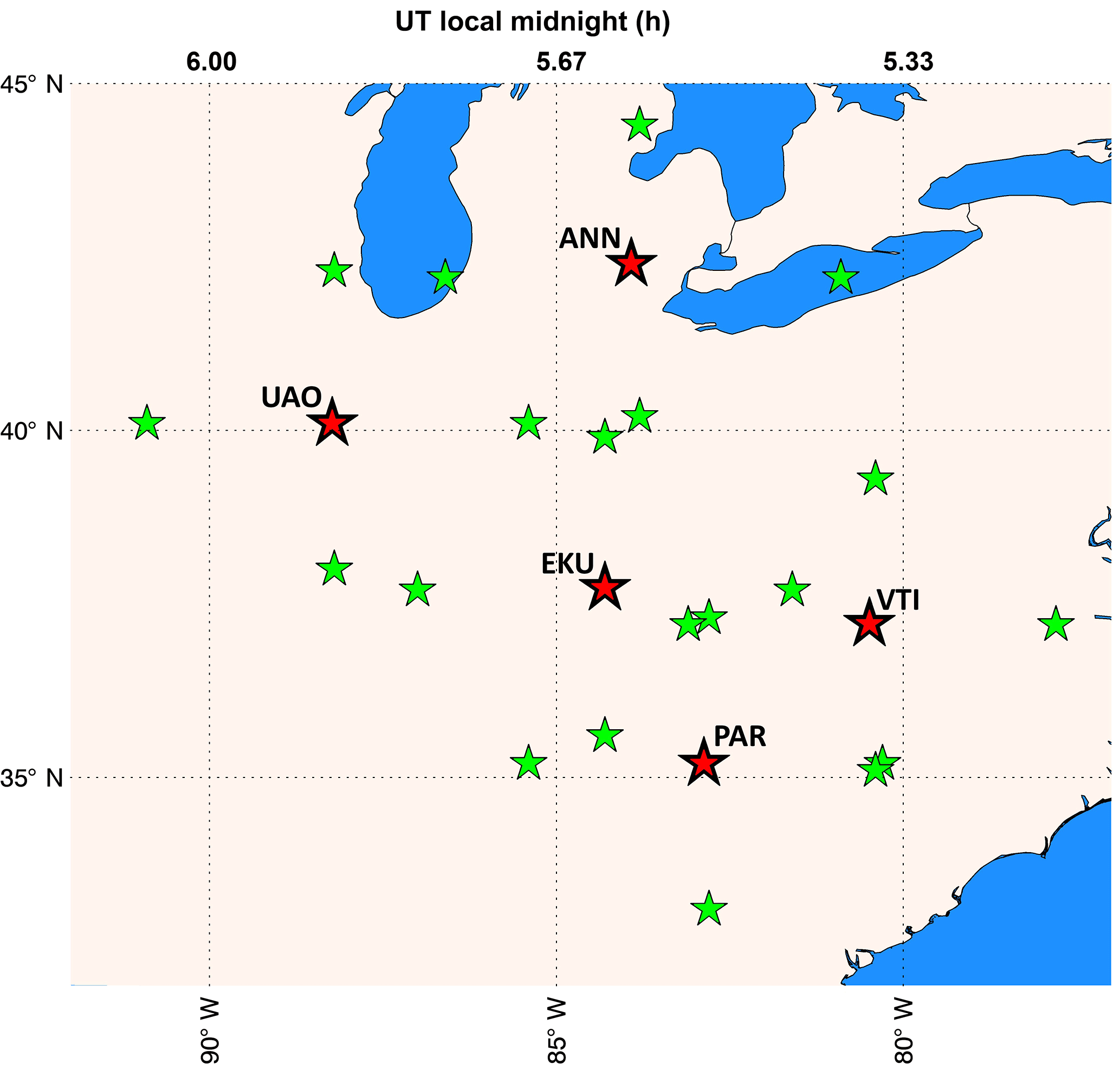
Figure 1NATION Cardinal Mode FPI observing configuration. Red and green stars mark the NATION site position and the measurement locations, respectively, for the North, East, South, and West directions assuming a 630 nm 250 km altitude. Red stars also represent the positions of the Zenith measurement. The top axis represents the local midnight in universal time.
2.3 Dynamic integration in image collection
The method of image collection called dynamic integration for each instrument in the NATION FPI network followed a procedure of image analysis, for which each measured spectrum is analyzed by the data collection computer to re-assess the need to increase or decrease the integration time for the next image collected by the CCD camera. The intent for this practice was to maintain a desired ratio of signal to noise from one image to the next so wind and temperature measurements are obtained with nearly the same uncertainty throughout the night. As the airglow signal becomes weaker or stronger during the night, the application of this procedure would increase or decrease the exposure time accordingly. This approach improves the cadence of measurements, which is integration time (between 20 and 720 s) times the number of look angles in the observation mode (typically the four cardinal positions and Zenith) that generally maintains the desired value of measured uncertainties as the 630 nm airglow intensity varies throughout the night. This typically represents an improvement in the number of measurement cycles per hour (from 2.5 to 4.5 cycles per hour) maintaining a fairly constant signal-to-noise ratio.

Figure 2(a) An example of the double MTM structure (black points) and two continuum thermal backgrounds assumed (linear and harmonic) for estimating the MTM amplitude (data for 31 August 2013). (b) Difference plots determined by subtractions of the background linear fit (red) and the harmonic fit (green) from the data points, respectively.
The normal temporal pattern of nighttime thermosphere temperatures is a cooling trend after sunset with a reversal to a warming trend starting several hours before dawn. Hence, in the absence of the MTM peak(s) one would expect the nighttime temporal behavior to be similar to a U-shaped temperature background featuring a valley. Because the breadth of the MTM structure is typically 2 h in local time, the determination of the MTM peak amplitude needs to account for a possible background curvature with local time. The method of determining the MTM amplitude that relies upon connecting the local minima with a straight line (linear fitting approach) will underestimate the amplitude in most cases. Figure 2 illustrates this method, which only uses the two local minima connected by red lines for each MTM feature.
In this paper a new approach to estimating the MTM amplitude is introduced that uses all of the temperature data instead of just the turning points of the temperature series that mark the starting (i.e., before the MTM peak) and ending (i.e., after the peak) points of the MTM peak profile (see Fig. 2 for differences between the approaches). This procedure uses a model in which the temperature data including the MTM are assumed to be the superposition of a background thermal variation and a Gaussian disturbance attributed to the MTM peak. This generally is a good approximation, given that small-scale temperature fluctuations are not related to the MTM. By first filtering the temperature data to remove the MTM structure, the overall nighttime background temperature variation is determined and subtracted from the observed set of FPI temperatures. This technique allows the MTM peak to be extracted as a set of temperature residuals relative to the background variation.
This technique is similar to the algorithm published by Martinis et al. (2013) for analysis of radar ion temperature data with an adaptation for the shorter time span of the FPI measurements. The idea is to manually ignore the MTM peaks (by excluding from the data set the temperature data from the local minimum before the MTM peak to the local minimum after the MTM peak) and fit a harmonic model to the remaining temperature data (without the MTM peaks) to determine the background thermal variation that will be subtracted from the data. It is assumed that the model fit to the thermal variation can be constructed with the combination of 8, 12, and 24 h harmonics. The residual values are then searched for the MTM peak by fitting a Gaussian profile (Eq. 2). The function used for the harmonic background removal model is given by
where a0 is the thermal background average, ai is the amplitude, bi is the phase, and τi is the period of each oscillation. An example of the differences in the results found using both approaches (linear fitting and the harmonic thermal background removal) can be seen in Fig. 2. In this figure the differences are ∼6 % (125.6 K vs. 118.4 K, an average difference of 6.6 K) for the primary MTM (around 03:00 LT) and ∼33 % (140.4 K vs. 93.5 K, with the average difference of 27.3 K) for the secondary MTM near 21:00 LT. Figure 3 also shows this technique applied to the monthly climatology plot of MTM events in the months of February 2012, 2013, 2014, and 2015. This figure displays both MTM features with amplitudes well above the uncertainty of the measurements, there represented by the vertical error bar.
The analysis of 846 nights was undertaken to study the frequency of the MTM and its double feature. These data came as a result of nearly 4 years (2012–2015) of observations by the NATION network in the eastern US. To find the MTM peak with accuracy it was necessary to use the harmonic background removal technique which allowed for the detection of the double MTM structure and the set of resulting residuals in the climatology study and the temperature interpolation case study. These results were combined with the method of inversion (Harding et al., 2015) to create 2-D temperature maps that were plotted together with a superposition of the measured wind field.
With regard to quality control of the data, the data showing any nonphysical wind speeds and temperatures, temperature and wind uncertainties larger than 50 K and 25 m −1, respectively, are not considered. The data are also filtered to remove periods of heavy cloud coverage. Also, note that when making reference to time, local time (LT) is the same as solar local time in the results displayed in Figs. 2, 3, 4, 8 and 9.
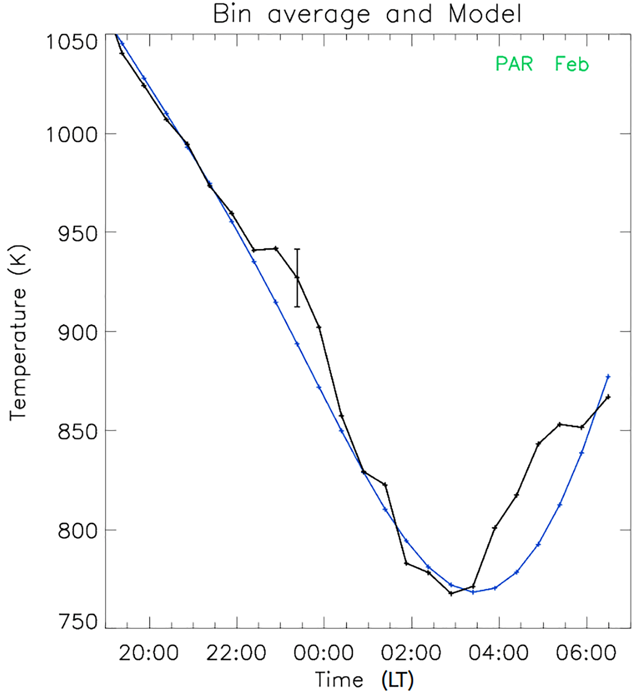
Figure 3Monthly climatology plot of the temperature data for nights with MTM events in the months of February 2012, 2013, 2014, and 2015. The blue curve represents the thermal background and the black curve is the averaged data for PARI. The vertical error bar is a representative depiction of the averaged measurement errors.
4.1 MTM double-peaked structure
To further investigate the seasonal variability of the MTM peak structure, the same harmonic background removal technique was applied to the monthly averaged temperature climatology. The monthly averaged climatology for the MTM results from the collection of all the nights with the presence of the MTM peak, averaged in half-hour time bins for a particular month. The temperature residuals, derived by subtracting the harmonic background model from the temperature data, are displayed in Fig. 4. The same figure shows the harmonic fitting for the peak times and the Gaussian fit for each peak as described by Eq. (2), where A0 is the amplitude, A1 is the LT of the center, and A2 is the width of each peak. It is evident that there is an annual behavior seen in the timing of the MTM, with the peak times being earlier in summer and later in winter months.
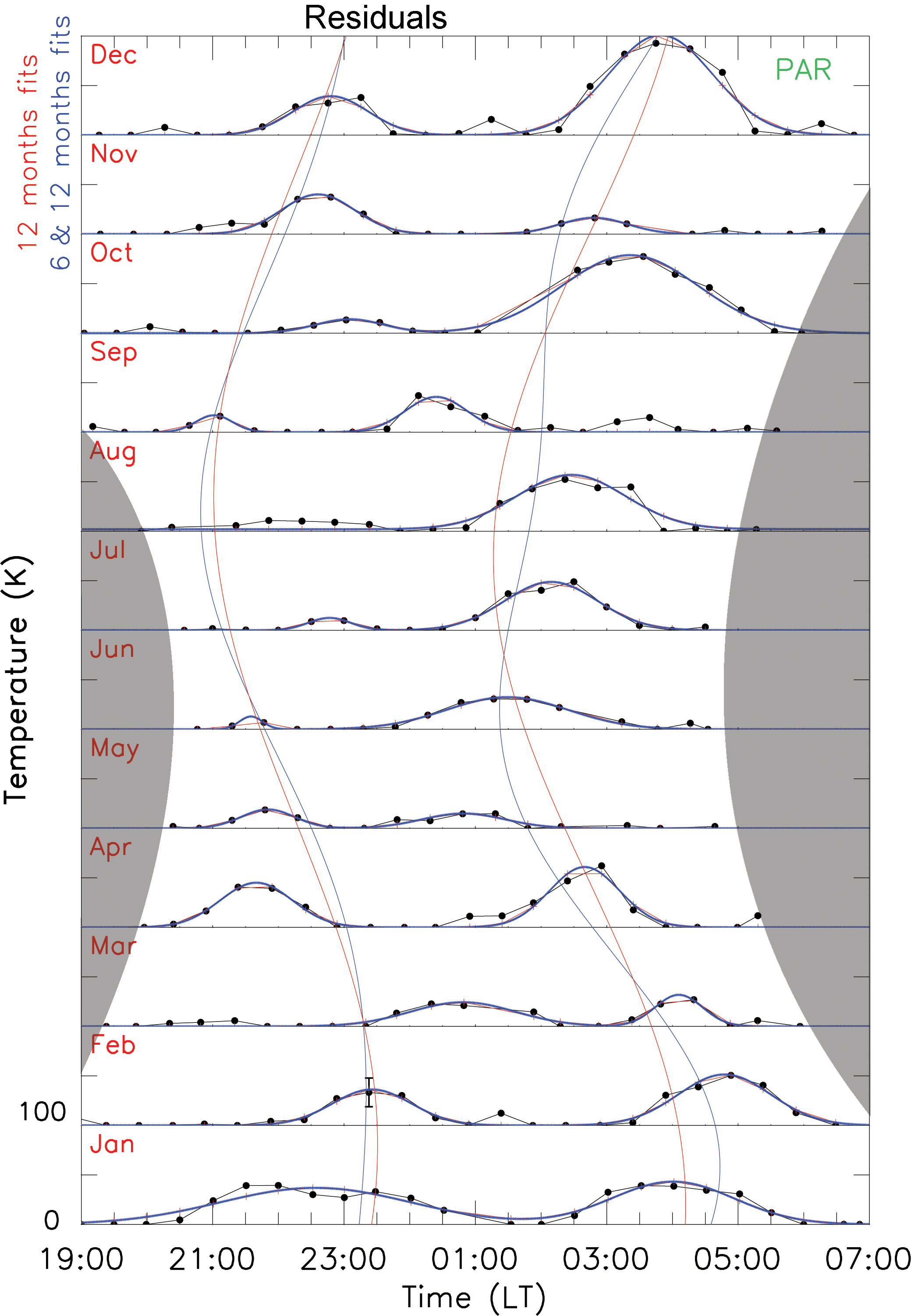
Figure 4Residuals resulting from the harmonic background removal technique (real data minus the background model from Eq. 1) and the monthly averages similar to Fig. 3. The annual (red) and annual and semi-annual (blue) oscillation fittings are plotted in the vertical orientation. Shaded areas represent day time periods. The black dots connected by lines are the temperature residuals and the horizontal blue curves are the least squares Gaussian fits for each of the MTM features (as described in Eq. 2).
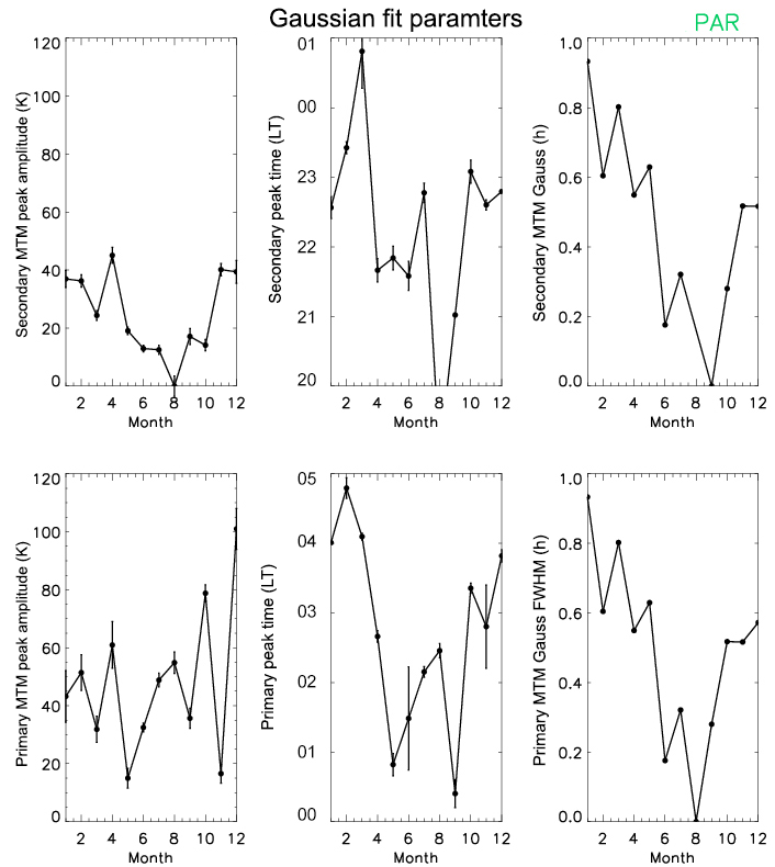
The averaged temporal difference between the two curves (primary MTM peak time fittings minus secondary MTM peak time fittings) is 04:28 ± 00:19 h. This result is consistent with what was found in the modeling work by Akmaev et al. (2009) and observed by Faivre et al. (2006). The averaged amplitudes for the primary and secondary MTM peaks are found to be 47 ± 24 and 24 ± 14 K, respectively. The coefficients of the Gaussian fits for each MTM peak and each month of the averaged MTM nights for PARI can be seen in Fig. 5. These coefficients for the Gaussian fit are shown in Eq. 2.
The MTM is a tidal wave generated near the geographic Equator and propagating northwestward (Northern Hemisphere) and southwestward (Southern Hemisphere) as a wake wave (Akmaev et al., 2009). That means that the primary and secondary MTM peaks (generated near the Equator around midnight and before twilight, respectively) will travel towards the poles and appear at different times relative to the latitude. The NATION network placement and latitude range allows both MTM peaks to be detected, especially for winter observations with its longer periods of darkness. The early night MTM (secondary MTM) makes its appearance in the southernmost NATION site near 23:00 LT and the primary MTM near 04:00 LT.
The other factor contributing to achieving detection of both MTM peaks is the fact that at mid-latitudes the nights are longer during the winter, allowing for measurements as early as 17:00 LT. However, during the summer months, when the nights are shorter, the bright continuum twilight background reduces the detectability of the secondary peak, as can be seen by inspection of Fig. 4.
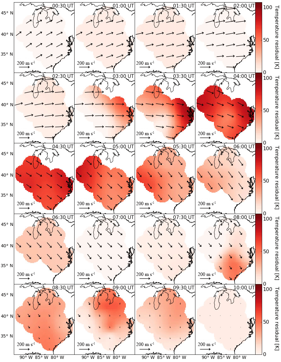
Figure 62-D temperature maps generated from the measurements with the harmonic thermal background removal technique for the night of 28 December 2013. Two clear MTM events are seen as suggested by the modeling work of Akmaev et al. (2009). The gray-shaded map represents the approximate local midnight in the middle of the NATION network.
4.2 Background extracted temperature interpolation
Figure 1 presents a map of the NATION Cardinal Mode measurement positions, showing that the NATION network offers a broad latitudinal and longitudinal coverage (about 1200 × 1200 km) of the Midwest continental region of the United States. Consequently, the possible analysis of the MTM peak and its large spatial structural characteristics, such as its direction of propagation and velocity, is expanded significantly as compared with the spatial extent observed by a single FPI observatory. This examination of the MTM spatial structure becomes more difficult if done using only the raw temperature data, where no emphasis is given to the MTM peaks, since the MTM thermal variation relative to the nighttime thermal variation represents a small fraction of the thermal background.
It is in this regard that the application of the harmonic thermal background removal procedure described by Eq. (1) becomes important. As shown above, the identification of the double MTM peak profile becomes clearer following the removal of the thermal background. Fitting a Gaussian to each of the two MTM peaks in the residual values yields accurate estimates for the amplitude and the peak time of occurrence. This procedure is also necessary in extracting the MTM peak structures for cases where smaller-scale oscillations, such as gravity wave activity, might be present in the data.
The large number of measurement positions in the NATION network allows for the detection of both MTM peaks (when present), in an inversion analysis similar to what was done by Harding et al. (2015) for the eastern Brazilian and NATION FPI networks for the winds. The authors used inversion theory to build an algorithm capable of estimating the wind fields. In this work, a modified version of this approach is applied to the temperature residuals to generate a temperature field in a manner similar to what was described by Harding et al. (2015) to calculate a horizontal wind field. This algorithm searches for the smoothest horizontal wind and temperature fields that fit the data within the data uncertainty. Figure 6 shows the result of the application of this technique for the night of 28 December 2013. It shows the appearance of both MTM structures and the corresponding change in the horizontal wind field behavior as a function of local time.
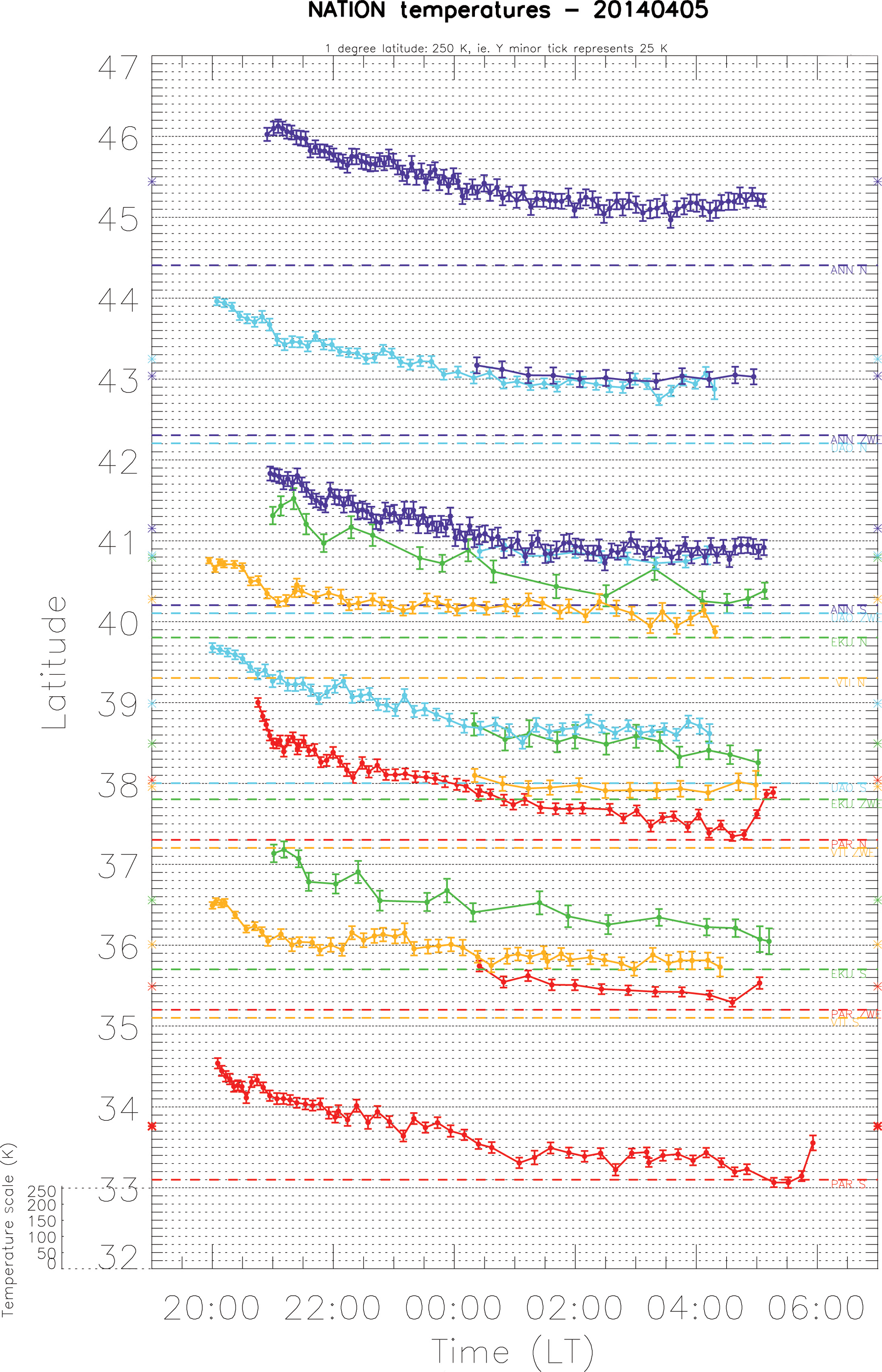
Figure 8NATION latitudinal temperature distribution graph for 5 April 2014, illustrating the lack of the double or single MTM structure. Each color represents the FPI temperature results of a NATION station with a set of three temperature lines (North, zonal, and South directions). From bottom to top, the line colors of red, orange, green, blue, and purple represent results for the PAR, VTI, EKU, UAO, and ANN NATION sites, respectively. The North, zonal, and South measurements are shifted to their respective latitudes, and the horizontal dashed baseline represents 800 K for that particular measurement. The magnitude of one degree latitude corresponds to a 250 K difference. The asterisks on the left and right vertical axes represent the temperature averages for each latitude set of measurements.

Figure 9Temperature distribution graph similar in style to Fig. 8, for 31 August 2013. These results illustrate the presence of the double MTM structure. The secondary peak near 22:00 LT in the southernmost measurement and the primary MTM peak near 03:00 LT.
Figure 6 shows results of this algorithm applied to the temperature residuals and winds. The propagation of the MTM is clearly seen to cross the NATION field of view from 03:00 to 06:00 UT and from 08:00 to 09:30 UT (UT used here due to the spatial coverage of the network; local midnight is approximately at 05:30 UT in the middle of the network). Both MTM peaks appear with winds in the southeastward direction and temperature maximums propagating predominantly to the westward and northwestward directions, respectively. However, the winds around the time of the secondary peak are faster and in the east–southeastward direction, while the primary MTM peak is associated with a slower wind field in the south–southeastward direction. This behavior is typical of the reversal of the winds occurring before the passage of the primary MTM peak (Akmaev et al., 2009).
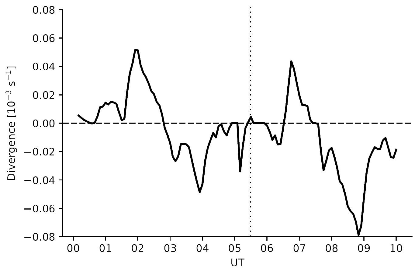
Further evidence for the double-peaked MTM structure comes from calculating the divergence of the wind field. The wind field is estimated at a 5 min cadence for the whole night over NATION at each time step. For every grid point, the divergence is calculated by comparing the residual value with its neighboring grid points, and the divergence is averaged over the entire grid. Figure 7 shows two periods of strong convergence at 04:00 and 08:30 UT, coincident with the peaks in the temperature seen in Fig. 6. Each period of convergence is preceded by a period of divergence.
The signature of the winds provides independent evidence for the occurrence at the mid-latitude MTM, as the convergence at 04:00 and 08:30 UT corresponds to the peaks in the temperatures, as would be expected from adiabatic heating. The divergence pattern displayed in Fig. 7 is mainly associated with the reversal of the meridional winds, resulting from the upward propagation of the tidal waves, as discussed by Akmaev (2011). The preceding period of divergence may be associated with the pressure bulge front (Herrero et al., 1985), but this cannot be conclusively explained without a larger number of observed nights with full coverage and perhaps measurements of pressure or vertical winds.
4.3 Statistics
Before describing the results of the statistical analysis of the mid-latitude MTM peak amplitude and time of occurrence based upon NATION data, we examine the definition of the MTM peak used in this analysis. The MTM peak structure is typically represented by primary and secondary peaks, with the primary peak occurring later with a larger amplitude. The time window of measurements for the NATION network would typically be in the range of 19:00–07:00 LT. We define the MTM peak as a significant increase in the temperature measurements compared to the thermal background. A threshold of 50 K or the measurement uncertainty (largest between the two criteria) is used to define such an increase as a MTM peak with the conditions that the MTM enhancement starts after 20:00 LT, continues for more than 1 h, propagates northward, and appears in at least three different measurement positions. That defines a MTM category used to collect the temperature increase events as well as the timing of the increase. The MTM-related brightness increase in the 630 nm intensities imposes another constraint. For an event to be in this MTM category, a brightness enhancement must also be evident in the FPI's 630 nm intensities (related to the brightness wave phenomenon discussed by Colerico et al., 2006). The MTM signature is also much larger in amplitude than the small-scale temperature fluctuations induced by gravity-wave activity and repeatable (each MTM peak happening in similar times from one night to the next).
The other two categories in the statistical analysis are the NO MTM category (clear absence of a defined maximum) and the inconclusive category (all nights with measurements from more than three stations that do not bring enough information to be able to categorize them as either MTM or NO MTM nights: typically nights with full moon or nights with long periods of cloud coverage). Out of a total number of 846 analyzed nights, 44 % were inconclusive, 43 % had no MTM peaks, and 13 % had the presence of the MTM in the temperature data.
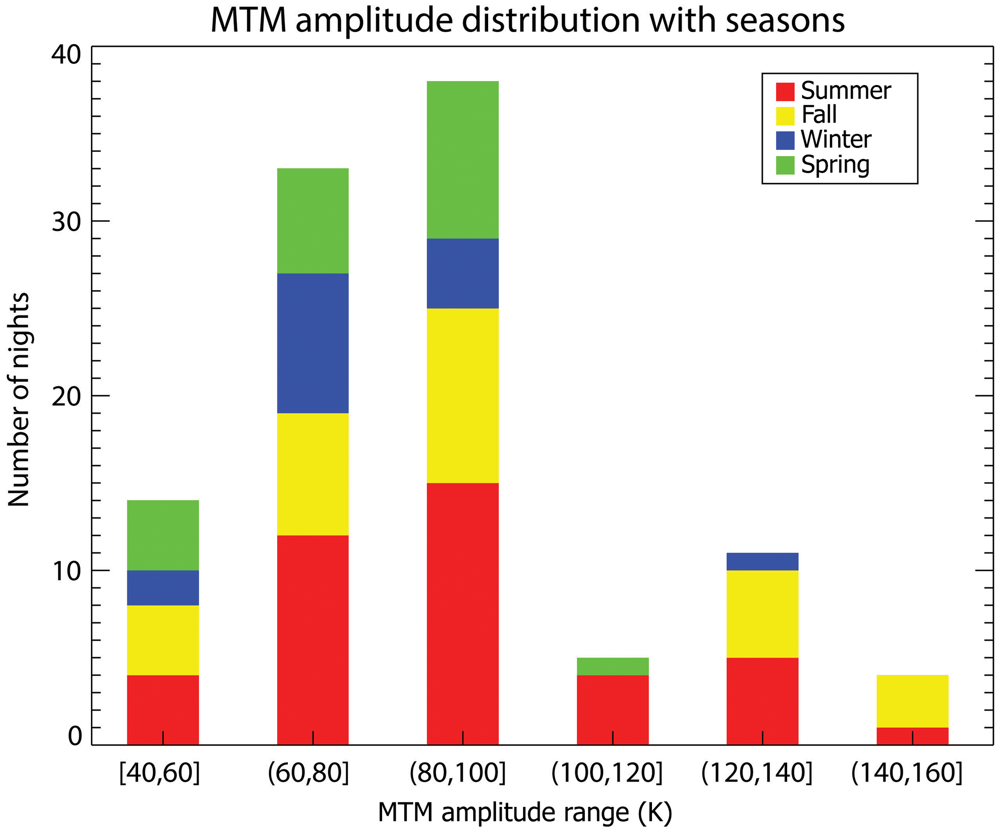
Figure 10MTM statistical distribution with regard to season and maximum amplitude for all the stations. The more frequent MTM amplitudes are found in the (60, 80] and (80, 100] ranges with 33 and 39 nights, respectively. MTM events with large amplitudes exceeding 120 K are occasionally seen (15 nights).
Figure 8 represents an example of a NO MTM night in a plot of the temperature data with the points shifted in latitude depending upon the latitude at the 250 km pierce point for each measurement direction. In the case of Figs. 8 and 9, the East, West, and Zenith measurements are averaged within a 30 min bin. These measurements have the same latitude and the longitude-related differences are averaged out since the East and West positions are equally spaced relative to the Zenith. The measurements for the North and South directions (indicated for each color/site as the top and bottom lines, respectively) are displayed in Figs. 8 and 9. These results do not have any bin averaging applied. Figure 9 displays an example of a MTM night that also shows the appearance of a double MTM structure feature.
Looking at the results of the statistical analysis with regard to the MTM amplitude (maximum peak), the MTM phenomenon shows no clear seasonal dependence for the range of latitudes that NATION measurements cover. This behavior can be observed with Fig. 10 (histogram with number of nights vs. MTM amplitude). The number of MTM nights for summer is slightly larger than the results seen for the other seasons, and any differences are negligible given the uncertainty in the analysis. Figure 10 also shows the the distribution of amplitudes, with the (80, 100] bin being the one with the largest number of occurrences (39 nights), corroborating the result observed in Table 1, which shows the MTM amplitude being 90.6±24.9 K.
Table 1Information about the MTM perturbation times (times for the beginning of the first peak and ending of the second) and maximum amplitude for all the stations.
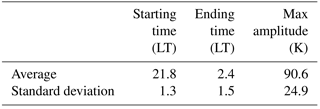
Figure 10 can also be used to show the MTM distribution with respect to the seasons. The seasonality of the MTM occurrence for the mid-latitude section is found to be slightly larger for summer (with 27 %) compared to the other seasons, with spring (with 18 %) showing the lowest frequency of the phenomenon occurrence. That behavior is consistent with modeling results and observations by Akmaev et al. (2009) and Martinis et al. (2013), respectively.
For NATION mid-latitudes the MTM phenomena appear to be quite active in the FPI data. As shown in Fig. 9, the MTM double-peaked structure appears at all sites within the NATION network, meaning that the MTM is seen as far as the most northern measurement by ANN North, which is located at 44.4∘ N and −83.8∘ W. It indicates that within the NATION latitudinal span the MTM phenomenon penetrates further toward the pole than the latitude of the southernmost appearance reported by Colerico et al. (2006) for the South American region.
The primary results of this work show the frequent detection of the MTM as a double-peaked phenomenon for the NATION network at mid-latitudes and within the American longitudinal sector. The reason that the secondary MTM peak is not generally seen at low latitudes is because its amplitude is weak and its occurrence would normally take place during the evening twilight where detection is more difficult. However, the time it takes the secondary peak to propagate to mid-latitudes proves enough temporal separation from the twilight to make it detectable. Furthermore, the results are consistent with what is shown by Akmaev et al. (2009), Akmaev (2011) and Faivre et al. (2006). The application of the NATION network to the study of the MTM phenomenon produced strong evidence of the MTM amplitude variability with northwestward propagation, which is the typical direction of propagation shown in Fig. 6 and previously observed near 39.0∘ for the Southern Hemisphere (Colerico and Mendillo, 2002; Colerico et al., 2006); this study confirms the presence of the MTM as far north as ANN North, corresponding to 44.4∘ N.
From a latitudinal standpoint, the MTM structure is much the same as what is observed at lower latitudes with regard to its direction of propagation. However, the amplitude is generally weaker and it appears with different morphology if compared to the analysis made for MTM events seen in the equatorial region (Figueiredo et al., 2017; Gong et al., 2016). The amplitude variation of the MTM as it propagates both poleward and westward may be mostly due to the difference in phases contributed by the superposition of the tidal modes Akmaev et al. (2009); Akmaev (2011), which changes the result of the tidal wave superposition in the mid-latitude region. Like any phenomenon in the upper atmosphere, the MTM is also subjected to partial or total dissipation processes. It will be important in future work to gain a better understanding of what the contributing factors causing the MTM to have such variation are (with respect to both time and space), possibly by examining TEC content and ionosonde data to search for a possible correlation between the MTM peak amplitude and the F-region plasma density.
It is understood that the formation of the mid-latitude MTM tidal wave is more influenced by higher-order tidal modes (Akmaev et al., 2009). Thus, the MTM peak structure does not have amplitudes as large as that found for the equatorial region observations. This is perhaps because the tidal forcing is stronger at low latitudes. Part of the reason why it was possible to observe the MTM peaks in the mid-latitude region was also the use of the harmonic background removal model. Its application enabled a more accurate investigation of the amplitude of the MTM and the development of the 2-D temperature residual maps for the NATION network. It was necessary to develop the harmonic thermal background removal technique in order to trace the MTM and avoid any underestimations as well as to enable the detection of such low amplitudes when compared to the thermal background. This approach estimates the MTM peak amplitude, with a difference of as much as 33 % when comparing it to the result of the linear fitting approach (Fig. 2).
The harmonic background removal model and the coverage of measurements from the NATION network enabled the imaging of the MTM feature using the process of the 2-D interpolation of the phenomenon. Figure 6 shows this result for the night of 28 December 2013. In this case the MTM can be detected with the presence of its double-peaked structure. The first peak, around 04:30 UT, has a strong westward component when compared with the primary MTM peak's northwestward behavior. It is also, for that particular night, longer lasting (about twice as long as the primary MTM) and with faster southeastern winds. The propagation speed of this peak is ∼120 m s−1.
The second MTM (primary), around 08:00 UT, has a northwestward propagation behavior with the northward component more pronounced. The wind field present in Fig. 6 suggests a flow towards the MTM peak, as the earlier peak, typical of the pressure bulge responsible for the generation of the MTM peaks, though with weaker winds. Another interesting result is the velocity of the primary MTM being ∼240 m s−1. The example associated with this night indicates the primary MTM moves faster in the background of weaker winds. Unfortunately similar analysis can only be done with the presence of clear skies in a vast area of the network, indicating that such analysis would be more feasible if done in a cloudless region such as the western US region.
With regard to its seasonality, the primary MTM peak shows a clear annual/semi-annual behavior in amplitude, appearing more often during summer with 27 % (around 9 % more than spring), which can be seen in Fig. 10. That behavior also appears in the phase of both MTM peaks. Both peaks exhibit annual/semi-annual behavior, as can be seen from Fig. 4. From the same figure, the time difference between the two vertical fittings is 04:28 ± 00:19 h, consistent with results from the WAM model (Akmaev et al., 2009). From the same figure we have 47.6 ± 24.8 and 24.9 ± 14.3 K for the average MTM amplitudes for the PARI site. Along with these averages we have the average of the maximum amplitude at 90.6 ± 24.9 K (accounting for all the sites), a starting time of 22:15 ± 01:19 LT, and an ending time of 02:53 ± 01:30 LT. No particular trend is found for the MTM with regard to its amplitude, as can be seen in Fig. 10.
Previous work on the MTM phenomenon has concentrated upon the equatorial and low-latitude results, and the question of the extent that the MTM phenomenology reached into higher latitudes has not been examined carefully. One reason for this might be attributed to the limitation associated with the application of a Fabry–Perot interferometer that has only a photomultiplier detector and observes only one interference order. Such instruments do not have sufficient sensitivity to observe the weak 630 nm nightglow with the necessary accuracy or the observing cadence to be able to detect the mid-latitude MTM phenomenon with confidence. Thus, it is likely for this reason that previous work associated with mid-latitude FPI observations did not report the successful detection of this phenomenon (Hernandez and Roble, 1976; Herrero and Spencer, 1982). Thus, the results presented in this paper illustrate how the new technology of FPI instrumentation features observations of multiple interference orders and the much higher quantum efficiency of the bare CCD detector has resulted in temperature observations with much improved quality regarding the reduction of observing errors and the increase in the number of samples per hour.
With the results reported in this paper, the MTM signature for the mid-latitude region shows a strong indication of the appearance of a double-peaked structure rather than a single peak as characteristic of the MTM results seen for lower latitudes. As stated before, these new results are consistent with the double MTM peak results found in the modeling work reported by Akmaev et al. (2009), Akmaev (2011), and Faivre et al. (2006). We also note that the application of a more suitable analysis technique would improve the accuracy of the MTM peak amplitude estimations (Hickey et al., 2014; Ruan and Kapali, 2013; Azeem et al., 2012).
By making a month-to-month binned average of the MTM nights and using the harmonic background removal model, the variation of the MTM characteristics with season become evident, as shown in Fig. 4. This climatology displays the fact that the extent of the NATION network coverage allows for the detection of both peaks. As the MTM double-peaked structure travels northward from the Equator, both MTM peaks become observable because of a systematic latitudinal-dependent phase shift of the MTM peak occurrence times to later local times with higher latitudes. Moreover, the longer winter nights help to make possible the observation of the MTM double-peaked structure.
The application of the harmonic background removal model for the night of 28 December 2013 shows the 2-D behavior of the MTM. The wake wave behavior of the MTM is well displayed in Fig. 6. It is also clear that the secondary and primary MTM peaks cross the NATION network, moving in somewhat different directions (northwest–west to northwest–north).
With regard to its general behavior, the mid-latitude MTM structure develops more often during the summer months (as shown in Fig. 10). However, the secondary maximum is more prominent during the winter months, as shown in Fig. 4. It is difficult to determine whether that behavior is due to the nature of the phenomenon or due to the difference between the duration of summer and winter nights. Nevertheless, the amplitude of the secondary MTM peak is stronger in the winter months, as illustrated by the results shown in Fig. 5 (top left graph).
Further work would be interesting to carry out for the same latitudinal region but with the NATION sites relocated to the southwestern United States. This relocation would provide better quality data year-round due to the clear skies found in this dryer region, which would improve the 2-D analysis of the MTM double-peaked structure in all seasons. Application of models such as general circulation models (WAM and TIEGCM) would help assess the similarity between the results from NATION and these model predictions. This analysis should help to understand the underlying day-to-day variability of the MTM double-peaked structure. Future work should also include a thorough investigation of the OH behavior, because the small OH contamination that exists for weak 630 nm airglow intensities may lead to a time-dependent error in the temperature measurements that could affect the background fit.
The data used in the analysis of this paper can be downloaded in the CEDAR Open Madrigal website http://cedar.openmadrigal.org/ (last access: March 2018). A simplified version of the data can be displayed on the Airglow at Illinois research group (University of Illinois at Urbana-Champaign) website http://airglow.ece.illinois.edu/Data/Calendar (last access: March 2018). For further reference/use of the wind, temperature and intensity data used in this paper, contact John W. Meriwether (meriwej@clemson.edu) and Jonathan J. Makela (jmakela@illinois.edu).
The authors declare that they have no conflict of interest.
The authors thank Marco Ciocca
(Eastern Kentucky University), Ben Goldsmith (Pisgah Astronomic Research Institute), and
Gregory Earle (Virginia Polytechnic
Institute and State University) and their teams for their contributions
regarding the support for the experiment. Support for the research was
provided by the National Science Foundation (NSF) grants to Clemson
University (AGS-1557472) and the University of Illinois (AGS-1452291). The
authors also acknowledge the support provided by the NSF (AGS-1360594 and
AGS-1552214).
The topical editor, Dalia
Buresova, thanks Rashid A. Akmaev, Kazuo Shiokawa, and one anonymous referee
for help in evaluating this paper.
Akmaev, R. A.: Whole atmosphere modeling: Connecting terrestrial and space weather, Rev. Geophys., 49, RG4004, https://doi.org/10.1029/2011RG000364, 2011. a, b, c, d, e
Akmaev, R. A., Wu, F., Fuller-Rowell, T. J., and Wang, H.: Midnight temperature maximum (MTM) in Whole Atmosphere Model (WAM) simulations, Geophys. Res. Lett., 36, L07108, https://doi.org/10.1029/2009GL037759, 2009. a, b, c, d, e, f, g, h, i, j, k, l, m
Arduini, C., Ponzi, U., Agneni, A., Laneve, G., and Mortari, D.: San Marco V Utafiti Drag Balance Instrument Data Processing and Accuracy Assessment, CRA Internal Document, 1992. a
Arduini, C., Broglio, L., and Ponzi, U.: Drag balance measurements in the San Marco D/L mission, Adv. Space Res., 13, 185–200, 1993. a
Arduini, C., Laneve, G., and Herrero, F. A.: Local time and altitude variation of equatorial thermosphere midnight density maximum (MDM): San Marco drag balance measurements, Geophys. Res. Lett., 24, 377–380, https://doi.org/10.1029/97GL00189, 1997. a
Azeem, S. I., Crowley, G., Noto, J., Kerr, R. B., Kapali, S., Riccobono, J., and Migliozzi, M.: Midnight Temperature Maximum Observations Over Millstone Hill, AGU Fall Meeting Abstracts, 2012. a
Bamgboye, D. K. and McClure, J. P.: Seasonal variation in the occurrence time of the equatorial midnight temperature bulge, Geophys. Res. Lett., 9, 457–460, https://doi.org/10.1029/GL009i004p00457, 1982. a
Behnke, R. A. and Harper, R. M.: Vector measurements of F region ion transport at Arecibo, J. Geophys. Res., 78, 8222–8234, https://doi.org/10.1029/JA078i034p08222, 1973. a
Colerico, M. and Mendillo, M.: The current state of investigations regarding the thermospheric midnight temperature maximum (MTM), J. Atmos. Sol-Terr. Phy., 64, 1361–1369, 2002. a, b
Colerico, M. J., Mendillo, M., Fesen, C. G., and Meriwether, J.: Comparative investigations of equatorial electrodynamics and low-to-mid latitude coupling of the thermosphere-ionosphere system, Ann. Geophys., 24, 503–513, https://doi.org/10.5194/angeo-24-503-2006, 2006. a, b, c, d
Faivre, M., Meriwether, J., Fesen, C., and Biondi, M.: Climatology of the midnight temperature maximum phenomenon at Arequipa, Peru, J. Geophys. Res.-Space, 111, A06302, https://doi.org/10.1029/2005JA011321, 2006. a, b, c, d
Figueiredo, C. A. O. B., Buriti, R. A., Paulino, I., Meriwether, J. W., Makela, J. J., Batista, I. S., Barros, D., and Medeiros, A. F.: Effects of the midnight temperature maximum observed in the thermosphere–ionosphere over the northeast of Brazil, Ann. Geophys., 35, 953–963, https://doi.org/10.5194/angeo-35-953-2017, 2017. a, b
Gong, Y., Zhou, Q., Zhang, S., Aponte, N., and Sulzer, M.: An incoherent scatter radar study of the midnight temperature maximum that occurred at Arecibo during a sudden stratospheric warming event in January 2010, J. Geophys. Res.-Space, 121, 5571–5578, https://doi.org/10.1002/2016JA022439, 2016. a, b
Greenspan, J.: Synoptic description of the 6300 Å nightglow near 78 west longitude, J. Atmos. Terr. Phys., 28, 739–745, 1966. a
Harding, B. J., Gehrels, T. W., and Makela, J. J.: Nonlinear regression method for estimating neutral wind and temperature from Fabry–Perot interferometer data, Appl. Opt., 53, 666–673, https://doi.org/10.1364/AO.53.000666, 2014. a
Harding, B. J., Makela, J. J., and Meriwether, J. W.: Estimation of mesoscale thermospheric wind structure using a network of interferometers, J. Geophys. Res.-Space, 120, 3928–3940, 2015. a, b, c
Hernandez, G. and Roble, R.: Direct measurements of nighttime thermospheric winds and temperatures, 1. Seasonal variations during geomagnetic quiet periods, J. Geophys. Res., 81, 2065–2074, 1976. a
Herrero, F. and Spencer, N.: On the horizontal distribution of the equatorial thermospheric midnight temperature maximum and its seasonal variation, Geophys. Res. Lett., 9, 1179–1182, 1982. a, b, c
Herrero, F., Mayr, H., Spencer, N., Hedin, A., and Fejer, B. G.: Interaction of zonal winds with the equatorial midnight pressure bulge in the Earth's thermosphere: Empirical check of momentum balance, Geophys. Res. Lett., 12, 491–494, 1985. a
Hickey, D. A., Martinis, C. R., Erickson, P. J., Goncharenko, L. P., Meriwether, J. W., Mesquita, R., Oliver, W. L., and Wright, A.: New radar observations of temporal and spatial dynamics of the midnight temperature maximum at low latitude and midlatitude, J. Geophys. Res.-Space, 119, 10499–10506, https://doi.org/10.1002/2014JA020719, 2014. a
Makela, J. J., Meriwether, J. W., Ridley, A. J., Ciocca, M., and Castellez, M. W.: Large-Scale Measurements of Thermospheric Dynamics with a Multisite Fabry-Perot Interferometer Network: Overview of Plans and Results from Midlatitude Measurements, Int. J. Geophys., 2012, 1–10, https://doi.org/10.1155/2012/872140, 2012. a
Makela, J. J., Harding, B. J., Meriwether, J. W., Mesquita, R., Sanders, S., Ridley, A. J., Castellez, M. W., Ciocca, M., Earle, G. D., Frissell, N. A., Hampton, D. L., Gerrard, A. J., Noto, J., and Martinis, C. R.: Storm time response of the midlatitude thermosphere: Observations from a network of Fabry-Perot interferometers, J. Geophys. Res.-Space, 119, 6758–6773, 2014. a
Martinis, C., Hickey, D., Oliver, W., Aponte, N., Brum, C., Akmaev, R., Wright, A., and Miller, C.: The midnight temperature maximum from Arecibo incoherent scatter radar ion temperature measurements, J. Atmos. Sol.-Terr. Phys., 103, 129–137, 2013. a, b
Mayr, H., Harris, I., Spencer, N., Hedin, A., Wharton, L., Porter, H., Walker, J., and Carlson, H.: Tides and the midnight temperature anomaly in the thermosphere, Geophys. Res. Lett., 6, 447–450, 1979. a
Meriwether, J., Faivre, M., Fesen, C., Sherwood, P., and Veliz, O.: New results on equatorial thermospheric winds and the midnight temperature maximum, Ann. Geophys., 26, 447–466, https://doi.org/10.5194/angeo-26-447-2008, 2008. a
Meriwether, J. W., Makela, J. J., Huang, Y., Fisher, D. J., Buriti, R. A., Medeiros, A. F., and Takahashi, H.: Climatology of the nighttime equatorial thermospheric winds and temperatures over Brazil near solar minimum, J. Geophys. Res., 116, A04322, https://doi.org/10.1029/2011JA016477, 2011. a
Nelson, G. and Cogger, L.: Dynamical behaviour of the nighttime ionosphere at Arecibo, J. Atmos. Terr. Phys., 33, 1711–1726, 1971. a
Ruan, H., L. J. D. X. Z. S. N. J., and Kapali, S.: Enhancements of nighttime neutral and ion temperatures in the F region over Millstone Hill, J. Geophys. Res.-Space, 118, 1768–1776, https://doi.org/10.1002/jgra.50202, 2013. a
Sastri, J. H., Ranganath Rao, H. N., Somayajulu, V. V., and Chandra, H.: Thermospheric meridional neutral winds associated with equatorial midnight temperature maximum (MTM), Geophys. Res. Lett., 21, 825–828, https://doi.org/10.1029/93GL03009, 1994. a
Sobral, J., Carlson, H., Farley, D., and Swartz, W.: Nighttime dynamics of the F region near Arecibo as mapped by airglow features, J. Geophys. Res.-Space, 83, 2561–2566, 1978. a
Spencer, N., Carignan, G., Mayr, H., Niemann, H., Theis, R., and Wharton, L.: The midnight temperature maximum in the Earth's equatorial thermosphere, Geophys. Res. Lett., 6, 444–446, 1979. a