the Creative Commons Attribution 4.0 License.
the Creative Commons Attribution 4.0 License.
 | 22 Mar 2018
Seasonal variations of thermospheric mass density at dawn/dusk from GOCE observations
Libin Weng
Jiuhou Lei
Eelco Doornbos
Hanxian Fang
Xiankang Dou
Thermospheric mass densities from the GOCE (Gravity field and steady-state Ocean Circulation Explorer) satellite for Sun-synchronous orbits between 83.5∘ S and 83.5∘ N, normalized to 270 km during 2009–2013, have been used to develop an empirical mass density model at dawn/dusk local solar time (LST) sectors based on the empirical orthogonal function (EOF) method. The main results of this study are that (1) the dawn densities peak in the polar regions, but the dusk densities maximize in the equatorial regions; (2) the relative seasonal variations to the annual mean have similar patterns across all latitudes regardless of solar activity conditions; (3) the seasonal density variations show obvious hemispheric asymmetry, with large amplitudes in the Southern Hemisphere; (4) both amplitude and phase of the seasonal variations have strong latitudinal and solar activity dependences, with high amplitude for the annual variation at higher latitudes and semiannual variation at lower latitudes; (5) the annual asymmetry and effect of the Sun–Earth distance vary with latitude and solar activity.
Keywords. Atmospheric composition and structure (pressure, density, and temperature)


Paetzold and Zschörner (1961) first reported the seasonal variations of thermospheric mass density through analysis of the drag data from several satellites. They found that the density variation has a 6-month periodicity, with maximum occurring in April/October and minimum occurring in January/July. Jacchia (1966, 1971) represented the seasonal variations of thermospheirc mass density through temperature functions, with amplitude as a function of height. Since then, the seasonal variations, particularly the annual and semiannual oscillations in the thermospheric mass density, have been widely studied and considered in the empirical models (Volland et al., 1973; Hedin et al., 1983, 1987; Fuller-Rowell et al., 1998; Picone et al., 2002; Bowman, 2004; Bowman et al., 2008a, b).
In the past decade, studies have been conducted to further examine the seasonal variations of thermospheric mass density. For instance, Guo et al. (2008) investigated the seasonal variations by using the Challenging Minisatellite Payload (CHAMP) accelerometer-derived density estimates normalized to 400 km, and they found that both the amplitude and phase of seasonal variations have significant latitudinal dependence and hemispheric asymmetry. Qian et al. (2009) examined the seasonal variations of thermospheric mass density and compositions associated with the eddy diffusion process from the lower thermosphere by using the Thermosphere Ionosphere Electrodynamic General Circulation Model (TIEGCM). Lei et al. (2012, 2013) comprehensively studied the seasonal density variations at 400 km by using the empirical orthogonal function (EOF) method and measurements from CHAMP and GRACE satellites during 2002–2010, and also discussed the Sun–Earth distance effect on the annual asymmetry through observations and simulations. Moreover, Liu et al. (2013) constructed an empirical model based on the CHAMP density estimates, and then discussed the solar dependence of the equinoctial asymmetry. Wang et al. (2014) investigated the seasonal variations of globally averaged thermospheric mass density at 400 km during 1996–2006 using an artificial neural network (ANN), and concluded that there exist strong linear relations between the annual/semiannual amplitudes and the solar activity. Emmert (2015) reviewed the studies of the thermosphere between 2000 and 2014, summarized several possible mechanisms to explain the seasonal variations, and demonstrated that further investigations are required to understand the seasonal variations of the thermosphere. Recently, Calabia et al. (2016) investigated the thermospheric mass density variations from GRACE data for the period 2003–2016 by using the principal component analysis (PCA) method, and discussed the annual variation for different local solar times (LSTs) and solar activities. Moreover, Salinas et al. (2016) found that the monthly global-mean CO2 profiles from TIMED/SABER have annual and semiannual oscillations (AO and SAO), but cannot explain the observed AO and SAO in the thermosphere. However, Jones et al. (2017) reported that simulations from the Thermosphere Ionosphere Mesosphere Electrodynamics General Circulation Model (TIMEGCM) demonstrated that the intra-annually varying eddy diffusion by the breaking gravity waves may not be the primary driver of the SAO in the thermosphere. Additionally, Mehta et al. (2017) expanded the EOF approach to three dimensions for the MSISE00 model, and provided global pictures of the seasonal density variations with a small number of modes and parameters.
Generally, most of the above observational studies focus on the CHAMP and GRACE data. The density estimates from these two satellites vary with the LST, height and also seasonal variations, besides solar and geomagnetic activity effects. However, delineating these variations is not always easy or possible. In this paper, we develop an empirical model and then study the seasonal variations of thermospheric mass density on the basis of GOCE (Gravity field and steady-state Ocean Circulation Explorer) retrieval data. The GOCE densities are different with the CHAMP and GRACE data, since the GOCE satellite provided the density only at the dawn/dusk LST sectors and at around 270 km. In other words, this Sun-synchronous satellite gave the observations at nearly constant dawn and dusk LST. Thus, the seasonal and solar activity variations in the GOCE data are not mixed with the LST. Additionally, the GOCE data at the lower altitude could increase our understanding of the seasonal variations of the lower thermosphere. In this study, we examine the seasonal variations of thermospheric mass density by our GOCE model, and further discuss the annual asymmetry and the effect of the Sun–Earth distance under different solar activity conditions.
2.1 GOCE density data
The GOCE satellite was launched on 17 March 2009 in near-circular and almost Sun-synchronous orbits, and could provide the thermospheric mass density in geographic latitude coverage from 83.5∘ S to 83.5∘ N (Doornbos et al., 2013). The LST positions of GOCE orbits were around dawn (06:15–07:10 LST) and dusk (18:15–19:10 LST) during satellite operations, and provided complete altitude between 275 and 230 km. Unlike the CHAMP and GRACE satellites, the GOCE satellite maintained its lower altitude through an ion propulsion array with variable thrust, and the mass density estimates were derived from the along-track acceleration through the drag (Doornbos et al., 2013). The observations covered the time period from 1 November 2009 through 20 October 2013, with a sampling rate of 10 s, which corresponded to a spatial resolution in the along-track direction of about 75 km. The retrieved GOCE mass densities are made available by the European Space Agency (https://earth.esa.int/web/guest/missions/esa-operational-missions/goce/goce-thermospheric-data).
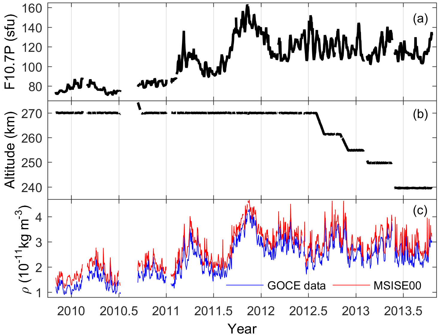
Figure 1(a) Solar flux index F10.7P, (b) daily mean GOCE height and (c) thermospheric mass density normalized to 270 km at dawn and dusk LST during 2009–2013.
Figure 1 displays the daily values of the solar flux index, GOCE altitude and thermospheric mass density normalized to 270 km. Figure 1a shows that the solar proxy F10.7P increases from ∼ 70 to ∼ 160 sfu with strong solar rotations (i.e., ∼ 27 days). Here, the solar F10.7P index is defined as F10.7P = (F10.7 + F10.7A) ∕ 2, where F10.7 is the daily solar flux proxy on the previous day and F10.7A is its 81-day average. In Fig. 1b, the daily mean height was about 270 km from November 2009 through July 2012, whereas it declined to a lower altitude after August 2012, and went ultimately down to about 240 km in May 2013.
To minimize the effect of different orbital altitudes, GOCE density estimates have been normalized to the constant altitude of 270 km by using the MSISE00 model according to the following equation:
where the subscript “M” stands for the MSISE00 model, and z is the GOCE satellite altitude. However, the estimated error incurred by this normalization would be small (Bruinsma et al., 2006). As we know, the MSISE00 is an empirical model maintained by the Naval Research Laboratory, and it computes total mass density as the sum of the main thermospheric compositions under the hypothesis of independent static diffuse equilibrium (Picone et al., 2002). Additionally, the main input parameters of this empirical model are time, location, daily F10.7, F10.7A and the 3-hourly geomagnetic index Ap array.
As shown in Fig. 1c, daily thermospheric mass densities normalized to 270 km at dusk LST are slightly greater than those at dawn LST, and their oscillations with the period of ∼ 27 days are consistent with the variations of solar flux in Fig. 1a. An interesting feature in Fig. 1c is that the GOCE densities in year 2012 have two peaks near equinoxes, with a primary minimum around the June–July months, although the solar activity does not undergo significant changes during this period. Further analysis of this feature will be given in the following sections.
2.2 GOCE density model
Daily GOCE density estimates normalized to 270 km altitude have decomposed the eigenvalues and eigenvectors using the following EOF analysis at the dawn and dusk LST sectors, respectively (Matsuo et al., 2002):
where EOFk(ϕ) is the kth EOF base function that changes with geographic latitude ϕ for each grid point at the center of the 5∘ latitudinal bin between 83.5∘ S and 83.5∘ N, which can represent the latitudinal distribution of the GOCE density. Moreover, αk(t) is the associated coefficient that varies as a function of day of year t, and m and ε represent the number of EOFs and the mean error. In Eq. (2), α1 × EOF1 denotes the mean field, while αk × EOFk represents the kth EOF. After calculation, the first three EOFs at dawn LST take up 99.14, 0.80 and 0.03 % of the total variability, while they are 99.38, 0.50 and 0.06 % at dusk LST. These results indicate that the EOF method can capture most of the observable features with only three orders. The first three orders of EOF base functions as well as the associated coefficients at the dawn and dusk LST sectors are shown in Fig. 2.
Additionally, the first three EOFs at the dawn and dusk sectors are parameterized using the following analytical function for each LST sector:
where , and the geographic latitude ϕ is in unit of degree. The obtained coefficients in Eq. (3) are shown in Table 1, and the fitting EOFk are also displayed in Fig. 2.
Table 1The coefficients of the first three EOFs fitted from Eq. (3) at the dawn and dusk LST sectors.
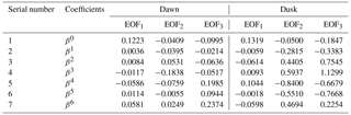
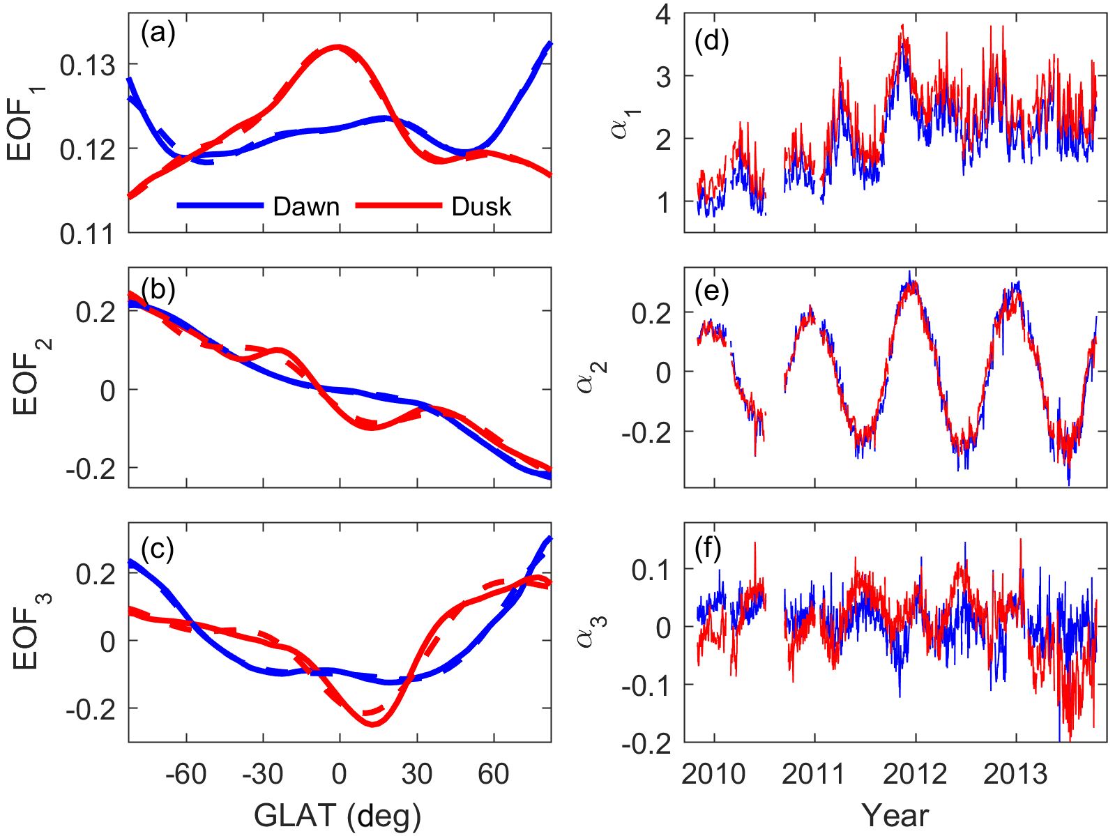
Figure 2(a, b, c) The first three orders of EOF base functions (solid line) and their fitting results from Eq. (3) (dashed line); (d, e, f) the associated coefficients (10−10 kg m−3) of GOCE data at the dawn and dusk LST sectors, respectively.
As seen in Fig. 2a, the EOF1 component means that the dawn densities peak in the polar regions, but the largest peaks in the dusk densities appear to be in the equatorial regions. The associated coefficients (Fig. 2d) illustrate the dominant solar effects, and the values are visibly greater than the second and third components. The EOF2 (Fig. 2b) mainly displays opposite patterns between the Northern Hemisphere and Southern Hemisphere, which are attributed to the annual variation of thermospheric mass density, and the associated coefficient (Fig. 2e) confirms the annual variation. Moreover, the EOF3 base functions and coefficients (Fig. 2c and f) contain the semiannual variations. Notably, the amplitudes of the first three EOF coefficients gradually increase from 2009 to 2013, which is consistent with the trend of solar flux F10.7P in Fig. 1a.
In this study, we discuss the seasonal variations of thermospheric mass density under the fixed solar and geomagnetic activity conditions, so the first three EOF coefficients in Fig. 2d–f are parameterized using the following function at each LST sector:
where F10.7P is the solar activity proxy at the Sun–Earth distance on the previous day, and Ap is the daily mean geomagnetic index. Additionally, Eq. (4) contains the seasonal variations associated with the annual/semiannual components. The coefficients in Eq. (4) are obtained from the linear regression of αk(t) in Eq. (2). Meanwhile, the coefficients in Eq. (4) at the dawn and dusk LST sectors are given in Table 2. Finally, we combine Eqs. (2)–(4) to develop a GOCE density model.
Table 2The coefficients of the EOF coefficients in Eq. (4) at the dawn and dusk LST sectors.
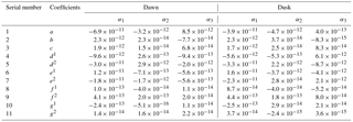
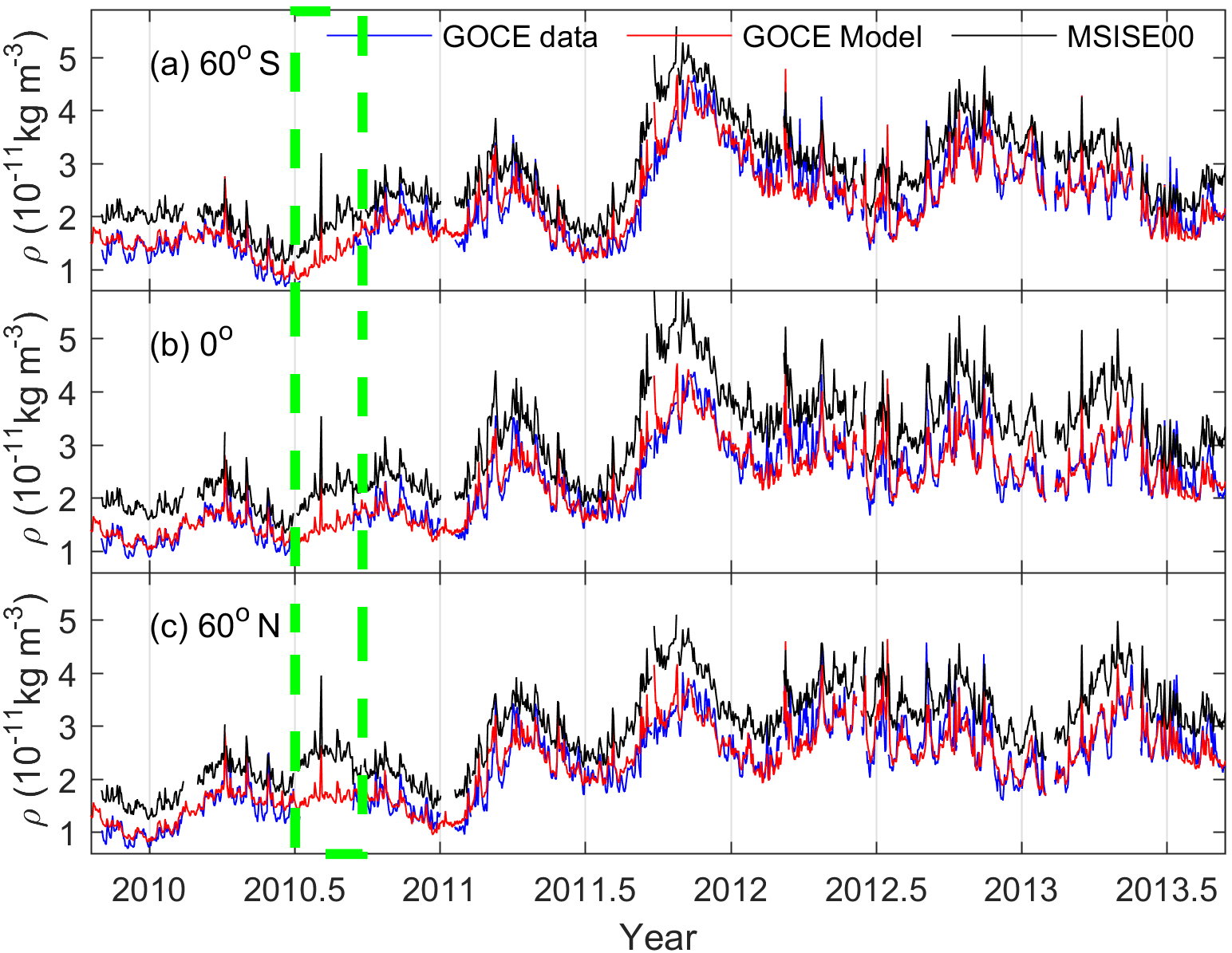
Figure 3The daily thermospheric mass density normalized to 270 km at dawn LST from GOCE data (blue line), and the corresponding results of our GOCE model (red line) and MSISE00 model (black line) at (a) 60∘ S, (b) 0∘ and (c) 60∘ N during 2009–2013. The dashed box (green line) shows the predicted mass density from our GOCE density model when the GOCE observations were not available.
Figure 3 shows the daily density estimates at dawn LST, similar results for the dusk side, and the calculated values from our GOCE model and the MSISE00 model at 60∘ S, 0∘, and 60∘ N, respectively. As expected, densities from our GOCE model are in good agreement with the observations. However, densities predicted from the MSIS00 model are greater than the GOCE observations, consistent with the results of Zhang et al. (2014) and Bruinsma et al. (2014, 2015, 2017). The mean ratios between the results of our GOCE and MSISE00 models and the observations are 1.012 and 1.334, with standard deviations of about 0.101 and 0.176, respectively. These results indicated that our GOCE model can reproduce the retrieved density better than the MSISE00 model. Moreover, as demonstrated in the green box in Fig. 3, our GOCE model can provide mass density predictions when the GOCE observations were not available.
In this section, we examine the seasonal variations of thermospheric mass density at dawn and dusk LST given by our GOCE model under different solar activity conditions. In our analysis, the Ap index is set to zero to minimize the effect of geomagnetic activity on the calculated density. In the following, densities from our GOCE model are hereafter referred to as the GOCE observations, and densities from the MSISE00 model are also included for the comparison. The daily solar proxy F10.7, F10.7A and Ap are used in these two empirical models.
As seen in Fig. 1a and c, the absolute GOCE density estimates generally increase with the increasing solar activity, and this is expected since the thermosphere is heated by the solar radiation and then expands to higher altitudes. Therefore, it is more appropriate to study the relative changes of thermospheric mass density to its annual mean in each geographic latitude bin. As shown in Fig. 4, the relative seasonal variations at the dawn and dusk LST sectors are similar under different solar activity conditions. The magnitudes of GOCE relative seasonal variations are smaller than those at dawn and dusk LST in Lei et al. (2012), who studied the thermospheric mass density at 400 km from the CHAMP and GRACE satellites, a higher altitude than the mean altitude of 270 km of the GOCE satellite. It suggests that the total mass density or the main constituents would play important roles in the different magnitudes of relative seasonal variations at different altitudes.
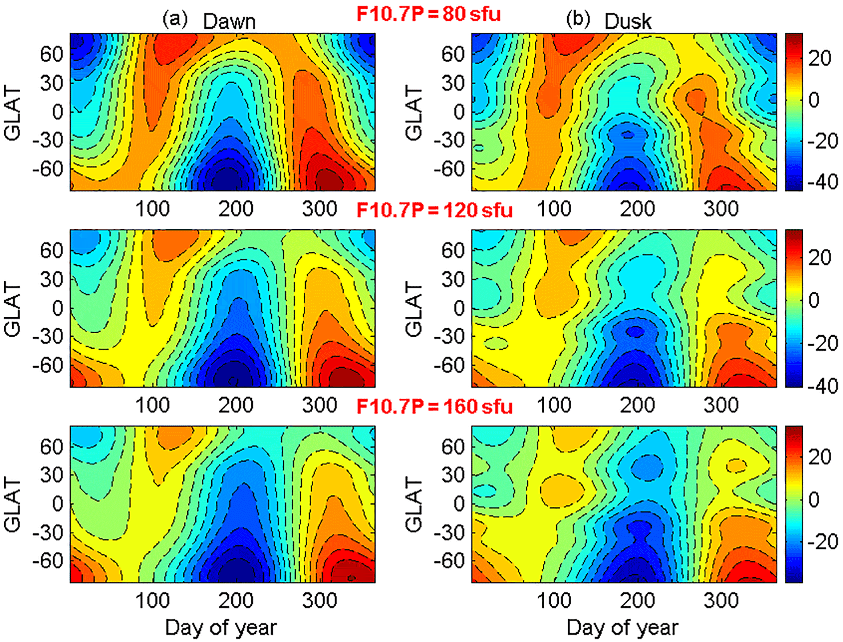
Figure 4Relative seasonal variations to its annual mean in units of percentage at dawn (a) and dusk LST (b) under different solar activity conditions.
Moreover, the relative seasonal variations show obvious hemispheric asymmetry, with larger values in the Southern Hemisphere than those in the Northern Hemisphere. In general, the mean amplitudes, i.e., the difference of maximum and minimum values, are about 65 and 45 % for the Southern Hemisphere and Northern Hemisphere, and this is presumably associated with the annual asymmetry as discussed later. Additionally, the largest negatively relative seasonal variations at dawn and dusk LST all appear in the southern polar regions around July. In the northern polar regions, there are two maxima peaks separated by a relative minimum around July, and the first maximum is greater than the second one. Moreover, only one maxima peak exists in the southern polar regions around December. Meanwhile, Figs. 6 and 13 in Calabia et al. (2016) also show that two maxima peaks are depicted in June in the Northern Hemisphere, but only one in December in the Southern Hemisphere. However, the underlying physical processes for this feature need further investigation. It should be noted that the seasonal densities from the MSISE00 model are generally in agreement with the GOCE observations in spite of some discrepancies in the detail features, and the results are similar to Fig. 5 in Lei et al. (2012). Thus, the results of the MSISE00 model are not shown in this paper.
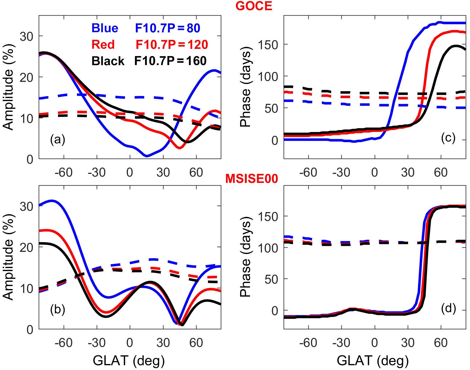
Figure 5(a, b) The relative amplitudes and (c, d) phases of annual (solid line) and semiannual (dashed line) components from (a, c) the GOCE observations and (b, d) the MSISE00 results at dawn LST under different solar activity conditions.
Figure 5 provides a quantitative comparison for the annual and semiannual components between the GOCE observations and the MSISE00 results at dawn LST under different solar activity conditions, and the amplitude and phase are calculated from Eq. (4). However, we only present the comparison at dawn LST in our study since the results are generally similar at dusk LST. In Fig. 5a, the GOCE annual variation is the dominant component at high latitudes of each hemisphere, particularly in the southern pole. In other words, GOCE annual amplitude has a hemispheric asymmetry, with much larger values in the Southern Hemisphere than that in the Northern Hemisphere. The GOCE annual amplitude decreases gradually from 82.5∘ S to about 35∘ N, and it increases with the solar activity. However, the annual amplitude increasing from 35 to 82.5∘ N exhibits an anti-correlation with the solar activity. Meanwhile, the GOCE semiannual variation becomes the stronger component at the lower latitudes, and it decreases with the solar activity. Notably, the variations of annual/semiannual amplitudes are generally larger from 80 to 120 sfu than that from 120 to 160 sfu. Comparatively, the MSISE00 results in Fig. 5b share similar latitudinal trends to the GOCE observations for both annual and semiannual amplitudes, but the annual component shows an opposite solar dependence. Nevertheless, the underlying physical processes for the solar activity dependence require further investigation.
The GOCE phase in Fig. 5c demonstrates that the annual variation usually peaks around local summer months and the semiannual variation has the maximum value at the equinoxes, with slight solar dependences. As shown in Fig. 5d, the phases of annual and semiannual components from the MSISE00 model are quite similar to those from GOCE observations, but without obvious solar dependences. However, our results in Fig. 5 are generally in agreement with the results of Fig. 6 in Lei et al. (2012).
The annual asymmetry of thermospheric density, larger in December solstice than that in June solstice, can be clearly seen in Figs. 4 and 5. It is defined as , with subscripts “Dec” and “Jun” denoting the December and June solstices, where represents the mean of Northern and Southern Hemisphere values at a given latitude. In Eq. (4), the solar flux at 1 AU would be multiplied by a factor obtained from the formula , where θ is equal to 2πt∕365, accounting for the Earth's orbital eccentricity effect on the Sun–Earth distance (see Lei et al., 2013).
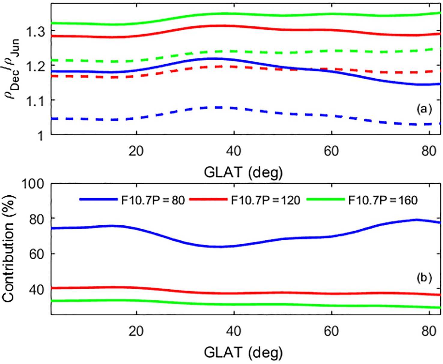
Figure 6(a) Annual asymmetry index R at dawn LST at each geographic latitude for different solar activities at 1 AU (solid line) and Sun–Earth distance (dashed line), and (b) the contributions of the Sun–Earth distance are also presented.
As seen in Fig. 6a, thermospheric annual asymmetry at dawn LST has significant latitudinal dependence, especially for the low solar activity, and it is greater at the middle latitudes, with similar results for the dusk side. After calculation, the mean annual asymmetry R values are 1.04, 1.17 and 1.21 for F10.7P = 80, 120 and 160 sfu at the Sun–Earth distance, but they become 1.17, 1.28 and 1.32 for the same solar activities at 1 AU. These results illustrate that the thermospheric annual asymmetry should be associated with the varying Sun–Earth distance. Actually, previous studies suggested that the difference of solar radiation associated with the difference of Sun–Earth distance between June and December would contribute to the annual asymmetry (Qian et al., 2012; Lei et al., 2013, 2016; Emmert, 2015; Calabia et al., 2016). Moreover, Fig. 6a also suggests that the Sun–Earth distance should be one of the most probable factors for the annual asymmetry, but the contributions from other processes need to be addressed in the future.
The contribution of the Sun–Earth distance is defined as , where R1 is the thermospheric annual asymmetry for solar flux at the Sun–Earth distance (solid lines in Fig. 6a), and R2 is the value for the solar flux at 1 AU (dash lines in Fig. 6a). Figure 6b shows the contributions under different solar activity conditions. Clearly, the Sun–Earth distance effect also depends on the latitude and solar activity. Our calculation revealed that the Sun–Earth distance effect can explain about 76 % of the December-to-June difference in the GOCE observations for F10.7P = 80 sfu, but the contribution is only 34 % for F10.7P = 160 sfu.

Figure 7(a) The latitudinal mean R from GOCE observations for solar flux at the Sun–Earth distance (dashed line) and 1 AU (solid line), and (b) the estimated contribution of the Sun–Earth distance under different solar activity conditions at the dawn and dusk LST sectors.
Figure 7a shows that the latitudinal mean R at the dawn and dusk LST sectors from GOCE observations has a positive nonlinear dependence with the solar activity. The R values are slightly larger at dusk LST for the low solar activity but slightly greater at dawn LST for the high solar activity. In Fig. 7b, the calculated contribution of the Sun–Earth distance effect is remarkably similar at the dawn and dusk LST sectors, being anticorrelated with the solar activity. Moreover, the variations of annual asymmetry and the contribution of the Sun–Earth distance from low to medium solar activities are greater than that from medium to high solar activities. This might be associated with the strongly nonlinear response of thermospheric mass density to the solar activity, with linear, saturated or magnified relations (Emmert et al., 2010; Niu et al., 2014). Moreover, the result in Fig. 7b shows that the Sun–Earth distance effect has less contribution to the annual asymmetry under the high solar activity conditions. However, long-term thermospheric observations are desired to further investigate this aspect.
In this paper, thermospheric mass densities from the GOCE satellite between 83.5∘ S and 83.5∘ N, normalized to 270 km during the period of 2009–2013, are used to study their seasonal variations at the dawn and dusk LST sectors, since this satellite mission is ideal for investigating the variations because of the lack of LST variations due to the Sun-synchronous nature of its orbit. A GOCE density model at 270 km has been constructed by using the EOF method at dawn and dusk LST, and it has been used to minimize the effects of solar and geomagnetic activities on the GOCE measurements. As a result, our GOCE model can well describe the variations of thermospheric mass density with latitude, season, and solar and geomagnetic activities.
The results in EOFs show that the dawn densities peak in the polar regions but the dusk densities maximize in the equatorial regions. Seasonal variations from GOCE observations can be seen from pole to pole, with similar patterns under different solar activity conditions. The relative seasonal variations show remarkable hemispheric asymmetry, and the mean amplitudes of the difference of maximum and minimum values are 65 and 45 % for the Southern Hemisphere and Northern Hemisphere, respectively. The thermospheric annual variation is dominant at high latitudes, especially in the Southern Hemisphere, whereas the semiannual variation tends to be the stronger component at the lower latitudes. Moreover, the GOCE amplitudes and phases of the annual/semiannual variations have significant latitudinal and solar dependences.
New findings on the annual asymmetry have revealed an interesting latitudinal dependence under the low solar activity conditions, with an asymmetric increase at middle latitudes. The annual asymmetry has a positive correlation with solar activity, but the contribution of the Sun–Earth distance is anticorrelated with solar activity, and this unexpected relationship needs to be further investigated. Finally, the variations of the annual asymmetry and the contribution of the Sun–Earth distance effect depend on solar activities, and the Sun–Earth distance has less contribution under the high solar activity condition.
Thermospheric density data derived from GOCE satellite are available online after registering at https://earth.esa.int/web/guest/missions/esa-operational-missions/goce/goce-thermospheric-data (GOCE+ Thermospheric Data, 2018).
The authors declare that they have no conflict of interest.
This work was supported by the National Natural Science Foundation of China
(41325017 and 41421063), the project of the Chinese Academy of Science
(KGFZD-135-16-013) and the Thousand Young Talents Program of China.
The topical editor, Andrew J. Kavanagh,
thanks Andres Calabia Aibar and one anonymous referee for help in evaluating
this paper.
Bowman, B. R.: The semiannual thermospheric density variation from 1970 to 2002 between 200 and 1100 km, Adv. Astronaut. Sci., 119, 1135–1154, 2004.
Bowman, B. R., Tobiska, W. K., Marcos, F. A., and Valladares, C.: The JB2006 empirical thermospheric density model, J. Atmos. Sol.-Terr. Phys., 70, 774–793, https://doi.org/10.1016/j.jastp.2007.10.002, 2008a.
Bowman, B. R., Tobiska, W. K., and Kendra, M. J.: The thermospheric semiannual density response to solar EUV heating, J. Atmos. Sol.-Terr. Phys., 70, 1482–1496, https://doi.org/10.1016/j.jastp.2008.04.020, 2008b.
Bruinsma, S., Forbes, J. M., Nerem, R. S., and Zhang, X.: Thermosphere density response to the 20–21 November 2003 solar and geomagnetic storm from CHAMP and GRACE accelerometer data, J. Geophys. Res., 111, A06303, https://doi.org/10.1029/2005JA011284, 2006.
Bruinsma, S. L.: The DTM-2013 thermosphere model, J. Space Weather Spac., 5, A1, https://doi.org/10.1051/swsc/2015001, 2015.
Bruinsma, S. L., Doornbos, E., and Bowman, B. R.: Validation of GOCE densities and evaluation of thermosphere models, Adv. Space Res., 54, 576–585, https://doi.org/10.1016/j.asr.2014.04.008, 2014.
Bruinsma, S., Arnold, D., Jäggi, A., and Sánchezortiz, N.: Semi-empirical thermosphere model evaluation at low altitude with GOCE densities, J. Space Weather Spac., 7, A4, https://doi.org/10.1051/swsc/2017003, 2017.
Calabia, A. and Jin, S.: New modes and mechanisms of thermospheric mass density variations from GRACE accelerometers, J. Geophys. Res., 121, 11191–11212, https://doi.org/10.1002/2016JA022594, 2016.
Doornbos, E., Bruinsma, S., Fritsche, B., Koppenwallner, G., Visser, P.,Van Den Ijssel, J., and de Teixeira de Encarnacõ, J.: ESA contract 4000102847/NL/EL, GOCE+ Theme 3: Air density and wind retrieval using GOCE data – Final Report, TU Delft, 2013.
Emmert, J. T.: Thermospheric mass density: A review, Adv. Space Res., 56, 773–824, https://doi.org/10.1016/j.asr.2015.05.038, 2015.
Emmert, J. T. and Picone, J. M.: Climatology of globally averaged thermospheric mass density, J. Geophys. Res., 115, A09326, https://doi.org/10.1029/2010JA015298, 2010.
Fuller-Rowell, T. J.: The “thermospheric spoon”: A mechanism for the semiannual density variation, J. Geophys. Res., 103, 3951–3956, https://doi.org/10.1029/97JA03335, 1998.
GOCE+ Thermospheric Data: GOCE Virtual Online Archive, European Space Agency (ESA), available at: https://earth.esa.int/web/guest/missions/esa-operational-missions/goce/goce-thermospheric-data, last access: 20 March 2018.
Guo, J., Wan, W., Forbes, J. M., Sutton, E., Nerem, R. S., and Bruinsma, S.: Interannual and latitudinal variability of the thermosphere density annual harmonics, J. Geophys. Res., 113, A08301, https://doi.org/10.1029/2008JA013056, 2008.
Hedin, A. E.: A revised thermospheric model based on mass spectrometer and incoherent scatter data: MSIS-83, J. Geophys. Res., 88, 10170–10188, https://doi.org/10.1029/JA088iA12p10170, 1983.
Hedin, A. E.: MSIS-86 Thermospheric Model, J. Geophys. Res., 92, 4649–4662, https://doi.org/10.1029/JA092iA05p04649, 1987.
Jacchia, L. G.: Density Variations in the Heterosphere, Ann. Geophys., 22, 75–85, 1966.
Jacchia, L. G.: Semiannual variation in the heteorosphere: A reappraisal, J. Geophys. Res., 76, 4602–4607, https://doi.org/10.1029/JA076i019p04602, 1971.
Jones Jr., M., Emmert, J. T., Drob, D. P., and Siskind, D. E.: Middle atmosphere dynamical sources of the semiannual oscillation in the thermosphere and ionosphere, Geophys. Res. Lett., 44, 12–21, https://doi.org/10.1002/2016GL071741, 2017.
Lei, J., Matsuo, T., Dou, X., Sutton, E., and Luan, X.: Annual and semiannual variations of thermospheric density: EOF analysis of CHAMP and GRACE data, J. Geophys. Res., 117, A01310, https://doi.org/10.1029/2011JA017324, 2012.
Lei, J., Dou, X., Burns, A., Wang, W., Luan, X., Zeng, Z., and Xu, J.: Annual asymmetry in thermospheric density: Observations and simulations, J. Geophys. Res., 118, 2503–2510, https://doi.org/10.1002/jgra.50253, 2013.
Lei, J., Wang, W., Burns, A. G., Luan, X., and Dou, X.: Can atomic oxygen production explain the ionospheric annual asymmetry?, J. Geophys. Res., 121, 7238–7244, https://doi.org/10.1002/2016JA022648, 2016.
Liu, H., Hirano, T., and Watanabe, S.: Empirical model of the thermospheric mass density based on CHAMP satellite observation, J. Geophys. Res., 118, 843–848, https://doi.org/10.1002/jgra.50144, 2013.
Matsuo, T., Richmond, A. D., and Nychka, D. W.: Modes of high-latitude electric field variability derived from DE-2 measurements: Empirical Orthogonal Function (EOF) analysis, Geophys. Res. Lett., 29, 1107, https://doi.org/10.1029/2001GL014077, 2002.
Mehta, P. M. and Linares, R.: A methodology for reduced order modeling and calibration of the upper atmosphere, Space Weather, 15, 1270–1287, https://doi.org/10.1002/2017SW001642, 2017.
Niu, J., Fang, H. X., and Weng, L. B.: Correlations between solar activity and thermospheric density, Chin. J. Space Sci., 34, 73–80, https://doi.org/10.11728/cjss2014.01.073, 2014 (in Chinese).
Paetzold, H. K. and Zschörner, H.: An annual and a semiannual variation of the upper air density, Pure Appl. Geophys., 48, 85–92, 1961.
Picone, J. M., Hedin, A. E., Drob, D. P., and Aikin, A. C.: NRLMSISE-00 empirical model of the atmosphere: statistical comparisons and scientific issues, J. Geophys. Res., 107, 1468, https://doi.org/10.1029/2002JA009430, 2002.
Qian, L. and Solomon, S. C.: Thermospheric density: an overview of temporal and spatial variations, Space Sci. Rev., 168, 147–173, https://doi.org/10.1007/s11214-011-9810-z, 2012.
Qian, L., Solomon, S. C., and Kane, T. J.: Seasonal variation of thermospheric density and composition, J. Geophys. Res., 114, A01312, https://doi.org/10.1029/2008JA013643, 2009.
Salinas, C. C. J. H., Chang, L. C., Liang, M., Yue, J., Russell, J., and Mlynczak, M.: Impacts of SABER CO2-based eddy diffusion coefficients in the lower thermosphere on the ionosphere/thermosphere, J. Geophys. Res.-Space, 121, 12080–12092, https://doi.org/10.1002/2016JA023161, 2016.
Volland, H. and Mayr, H. G.: Note on the semiannual effect in the thermosphere, J. Geophys. Res., 78, 3991–3994, 1973.
Wang, S., Weng, L., Fang, H., Xie, Y., and Yang, S.: Intra-annual variations of the thermospheric density at 400 km altitude from 1996 to 2006, Adv. Space Res., 54, 327–332, https://doi.org/10.1016/j.asr.2013.12.011, 2014.
Zhang, J. T., Forbes, J. M., Zhang, C. H., Doornbos, E., and Bruinsma, S. L.: Lunar tide contribution to thermosphere weather, Space Weather, 12, 538–551, https://doi.org/10.1002/2014SW001079, 2014.