the Creative Commons Attribution 4.0 License.
the Creative Commons Attribution 4.0 License.
 | 16 Mar 2018
A major event of Antarctic ozone hole influence in southern Brazil in October 2016: an analysis of tropospheric and stratospheric dynamics
Gabriela Dornelles Bittencourt
Caroline Bresciani
Damaris Kirsch Pinheiro
José Valentin Bageston
Nelson Jorge Schuch
Hassan Bencherif
Neusa Paes Leme
Lucas Vaz Peres
The Antarctic ozone hole is a cyclical phenomenon that occurs during the austral spring where there is a large decrease in ozone content in the Antarctic region. Ozone-poor air mass can be released and leave through the Antarctic ozone hole, thus reaching midlatitude regions. This phenomenon is known as the secondary effect of the Antarctic ozone hole. The objective of this study is to show how tropospheric and stratospheric dynamics behaved during the occurrence of this event. The ozone-poor air mass began to operate in the region on 20 October 2016. A reduction of ozone content of approximately 23 % was observed in relation to the climatology average recorded between 1992 and 2016. The same air mass persisted over the region and a drop of 19.8 % ozone content was observed on 21 October. Evidence of the 2016 event occurred through daily mean measurements of the total ozone column made with a surface instrument (Brewer MkIII no. 167 Spectrophotometer) located at the Southern Space Observatory (29.42∘ S, 53.87∘ W) in São Martinho da Serra, Rio Grande do Sul. Tropospheric dynamic analysis showed a post-frontal high pressure system on 20 and 21 October 2016, with pressure levels at sea level and thickness between 1000 and 500 hPa. Horizontal wind cuts at 250 hPa and omega values at 500 hPa revealed the presence of subtropical jet streams. When these streams were allied with positive omega values at 500 hPa and a high pressure system in southern Brazil and Uruguay, the advance of the ozone-poor air mass that caused intense reductions in total ozone content could be explained.
Keywords. Atmospheric composition and structure (middle atmosphere – composition and chemistry)


Ozone (O3) is the most important trace gas constituent of the stratosphere (Seinfeld and Pandis, 2016), which along with water vapor (H2O) and carbon dioxide (CO2) is responsible for the energy balance of the planet. This element plays a key role in supporting life on the surface of Earth due to its ability to absorb ultraviolet (UV) radiation (Salby, 1996; Dobson, 1968). Most of the atmospheric ozone content (about 90 %) is concentrated in the stratosphere between 15 and 35 km of altitude (London et al., 1985) in the region known as the ozone layer. Because of the great abundance of this compound at these altitudes, the real concentration of ozone in a particular region on Earth is mainly determined by the southward transport of this compound in the stratosphere (Gettelman et al., 2011).
High concentrations of ozone in the polar regions rather than in the equatorial region (where there is greater production of ozone) are due to a special type of southward transport known as the Brewer–Dobson circulation. In this phenomenon, air masses of stratospheric origin are transported horizontally from the equator to the poles (Brewer, 1949; Dobson, 1968). The southward transport of stratospheric ozone is one of the essential factors for the concentration of this atmospheric constituent in certain regions of the planet (Ploeger et al., 2012). Ozone has been extensively studied by calculating absolute potential vorticity (APV), which is correlated to the transport of chemical constituent traces, such as ozone, nitrous oxide, and water vapor on isentropic surfaces in the lower stratosphere. Potential vorticity (PV) acts as a tracer of large-scale air-mass dynamics and behaves as a material surface where the potential temperature is conserved (Hoskins et al., 1985). In the lower region of the stratosphere, the lifespan of O3 molecules is longer, which allows them to be used as tracers in the study of air-mass flows in the stratosphere–troposphere exchange (Bukin et al., 2011).
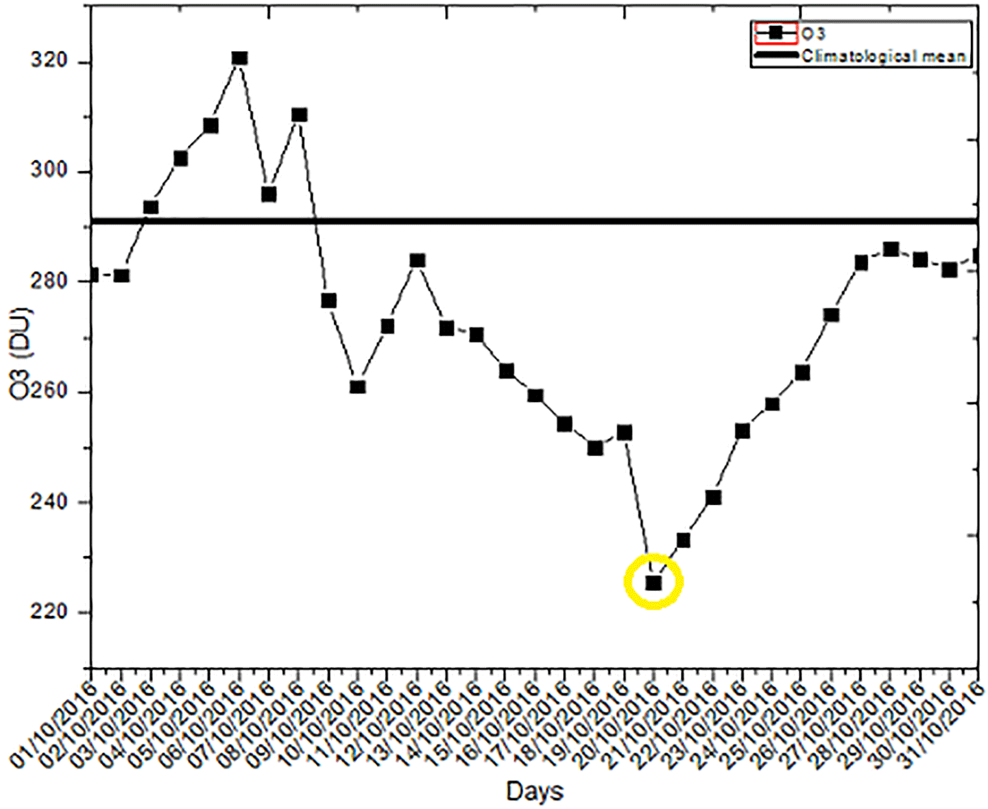
Figure 1Daily mean of the total ozone column in October showing the reduction analyzed (yellow circle) and the climatological mean for the reference month (continuous black line).
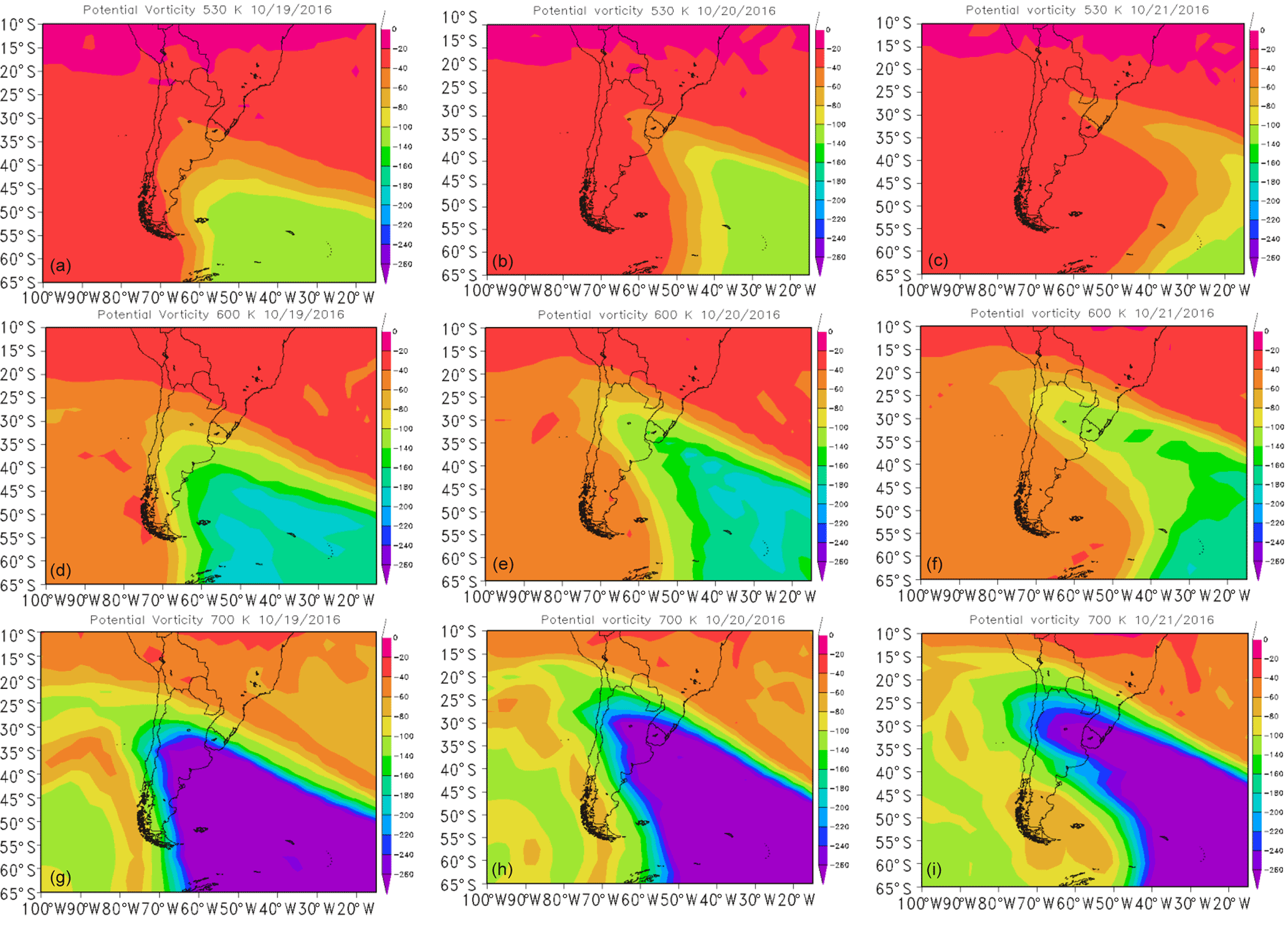
Figure 2Potential vorticity for the potential temperature levels of 530 K (a, b, and c), 600 K (d, e, and f), and 700 K (g, h, and i). The color scale ranges from 0 to 260 and shows the increase in APV.
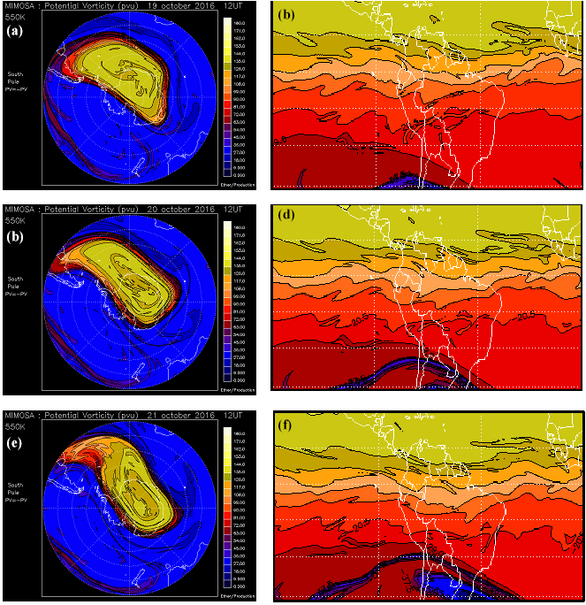
Figure 3MIMOSA model for the analysis period showing the connection between the ozone hole and the study region.
Chubachi (1984) and Farman et al. (1985) have reported massive destruction of ozone content during the spring in the Southern Hemisphere, which is currently known as the Antarctic ozone hole. This temporary destruction directly influences ozone content in polar regions and their vicinities due to the passage of the polar vortex border over these regions, causing drastic reductions in ozone content and increasing levels of UV radiation that reaches the surface of Earth (Casiccia et al., 2008). Additionally, these effects can also reach regions of medium and low latitudes, causing temporary decreases in total ozone column and abrupt increases in UV radiation levels. Ozone-poor air masses are released from the interior of the Antarctic polar vortex near the edge of the ozone hole in a phenomenon known as the secondary effect of the Antarctic ozone hole (Marchand et al., 2005). This phenomenon results in a temporary drop of ozone content, which was first observed by Kirchhoff et al. (1996) in southern Brazil.
Climatic conditions in southern Brazil are strongly influenced by transient meteorological systems, including frontal systems, which are an influence not observed in any other regions of the country (Reboita et al., 2010). These frontal systems bring strong western winds at high tropospheric levels (between 9 and 13 km of altitude) called subtropical or polar jet currents. Such currents play an important role in the vertical distribution of ozone and are considered the main tropospheric pattern directly linked to the transport of ozone from the stratosphere to the troposphere. Thus, the ozone total column (OTC) depends on meteorological dynamic factors, which in turn depend on seasonal variations at a synoptic scale (Bukin et al., 2011). Understanding the patterns of both influences has become increasingly important to understand how these events occur and behave. Additionally, there is possibility of a linkage of some meteorological phenomena during events of influence of the Antarctic ozone hole (Ohring et al., 2010). Therefore, the present study aimed to analyze stratospheric and tropospheric dynamics during an extreme event of influence of the Antarctic ozone hole that reached southern Brazil in October 2016. According to this information, the results presented here show the importance of studying and analyzing these events of influence of the Antarctic ozone hole, mainly on populous regions such as Uruguay and southern Brazil.
2.1 Study region, instruments, and methodology
The main region of study was the central region of the state of Rio Grande do Sul, Brazil. The main surface instrument to measure ozone levels was the Brewer MkIII no. 167 Spectrophotometer, which is located at São Martinho da Serra at the Southern Space Observatory – OES/INPE (29.4∘ S, 53.8∘ W; 488.7 m).The Brewer Spectrophotometer is an automated surface instrument that measures global solar radiation in the type B ultraviolet (UV-B) band for five wavelengths (306.3, 310.1, 313.5, 316.8, and 320.1 nm), where every 0.5 nm determines the spectral distribution of the incident radiation intensity. This instrument enables the deduction of the total column of the following atmospheric gases: ozone (O3), sulfur dioxide (SO2), and nitrogen dioxide (NO2). Data from the Ozone Monitoring Instrument (OMI) satellite were also used for the same location of analysis for days since no surface instruments for the measurement were available from OMI-ERS2/NASA (2017). The OMI satellite instrument was launched in July 2004 on board the ERS-2 satellite. It continued the TOMS satellite records that ended activity in 2005 for the OTC and other atmospheric parameters related to ozone, such as NO2 and SO2. This instrument can distinguish between different types of aerosols, such as smoke, dust, and sulfates. In addition, the instrument measures pressure and cloud cover. Peres et al. (2017) reported good correlation between these two types of data used, surface instrument (Brewer) and satellite instrument (OMI), which further confirms the reliability of these data for the study region.
For the analyses of tropospheric and stratospheric dynamics, daily data from the European Centre for Medium-Range Weather Forecasts (ECMWF) platform were used. These data were taken from ECMWF/ERA-Interim (Dee et al., 2011). Hence, analyses of tropospheric dynamics and meteorological fields were generated with aid of the public domain software Grid Analysis and Display System (GrADS). The meteorological fields generated are as follows: (i) the pressure at mean sea level and thickness between 1000 and 500 hPa, (ii) the horizontal wind cut at 250 hPa and omega values at 500 hPa, and (iii) a vertical section of the atmosphere of potential temperature (in Kelvin) and wind (in m s−1) for the longitude of 54∘ W. In order to complement these data, GOES satellite images available at CPTEC/INPE (2017) were analyzed in the thermal infrared channel and also in the water vapor channel in order to better verify the tropospheric patterns during the days of influence events of the Antarctic ozone hole.
Analyses of stratospheric dynamics also included daily data available on the ECMWF/ERA-Interim platform where absolute potential vorticity (APV) fields were analyzed on isentropic surfaces for three different potential temperature levels: 530, 600, and 700 K (Kelvin). The potential vorticity (PV) acts as a dynamic tracer of large-scale air masses where the potential temperature is conserved and used as a horizontal coordinate (HOSKINS et al., 1985). Thus, PV is used in studies that correlate potential vorticity with chemical constituents such as ozone, water vapor, and nitrous oxide on isentropic surfaces (adiabatic surfaces where the potential temperature remains constant as temperatures and pressure vary) in the lower troposphere (Schoeberl et al., 1989). This type of analysis aims to verify whether the air masses are originated in the Antarctica region, showing an increase in APV considering the previous days of the event, or in the equatorial region in the case of an APV decrease (Semane et al., 2006). Images from the OMI satellite (OMI-ERS2/NASA, 2017) were also used.
2.2 Stratospheric analysis
The first step was to extract the daily average of the total column of ozone obtained from ground-based and satellite instruments mentioned above. We identified days that the average daily value of the total ozone column were lower than the climatological average of the month analysis −1.5 of its standard deviation (μi–1.5σi). Herein, μi is the climatological average for the month of interest, σi is the standard deviation, and −1.5 is the criterion chosen from normal frequency distribution tests (Wilks et al., 2006). The climatological mean used in this study was from 1992 to 2016. The climatological mean and standard deviation for October at the station of the Southern Space Observatory (OES/INPE) was 291.0 and 10.3 DU, respectively.
After identifying days of reduced ozone concentration, isentropic analysis of APV was carried out from ECMWF reanalysis data for one day before and one day after the event. Maps (Fig. 2) were generated for different levels of potential temperature: 530, 600, and 700 K. An improvement in the ozone-poor air mass for Uruguay and southern Brazil was observed. Ozone depletion was observed to be more evident at MIMOSA (Modélisation Isentrope du transport Mésoéchelle de l'Ozone Stratosphérique par Advection). MIMOSA is a high-resolution model developed by the Service d'Aéronomie in the framework of the European METRO (MEridional TRansport of Ozone in the lower stratosphere) project. A complete description of MIMOSA was published by Hauchecorne et al. (2001). The model principle is based on the advection of Ertel potential vorticity (EPV) by using meteorological fields from ECMWF or NCEP data. In the lower stratosphere, EPV is assumed to be conservative on isentropic surfaces for periods of about one week (Orsolini, 1995). For longer periods, diabatic transport across isentropic surfaces occurs due to radiative cooling and warming of air masses; thus, the diabatic advection term should be taken into account in the EPV equation (Bencherif et al., 2003; Semane et al., 2006). The MIMOSA model produces advected APV files at different isentropic surfaces and for global spatial coverage. Although the MIMOSA APV is not the real EPV but a quasi-passive potential vorticity, it gives a consistent view of isentropic transport of air masses due to planetary wave breaking in the stratosphere (Bencherif et al., 2007). For the present case study, APV fields from MIMOSA were used to follow air-mass transport before and during the low ozone event observed on 20 October 2016.
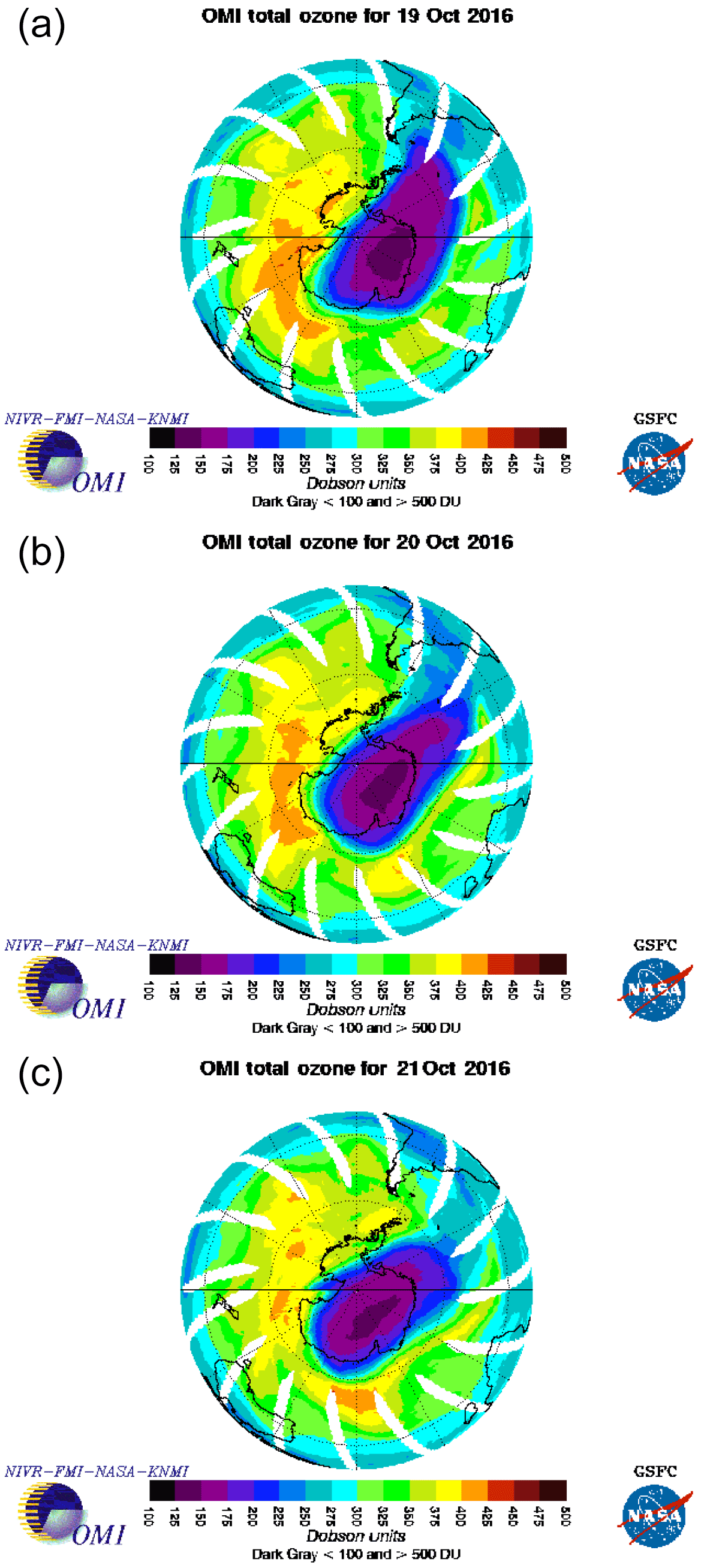
Figure 4Image of the OMI satellite showing the influence of the ozone hole for southern Brazil.
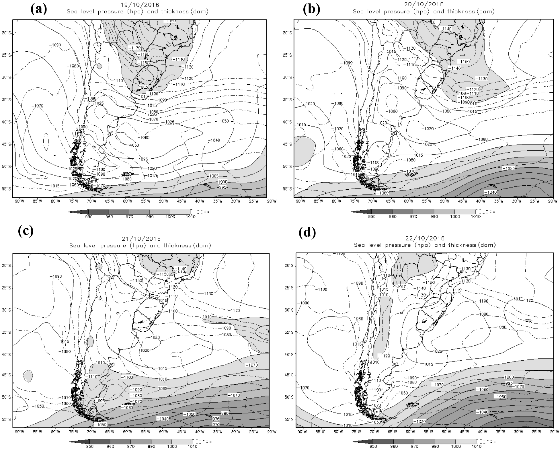
Figure 5Average daily pressure fields at medium sea level and thickness between 1000 and 500 hPa from 19 to 22 October. Shaded areas show pressure levels and dotted lines the thickness.

Figure 6Horizontal cut showing jet streams at 250 hPa and omega values at 500 hPa. The shaded area reveals jet streams showing maximum velocity in m s−1. The yellow triangle represents the study region.
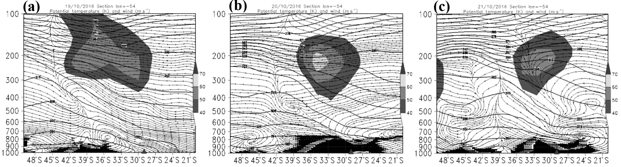
Figure 7Vertical cut between 1000 and 100 hPa showing the presence of jet streams at high levels.
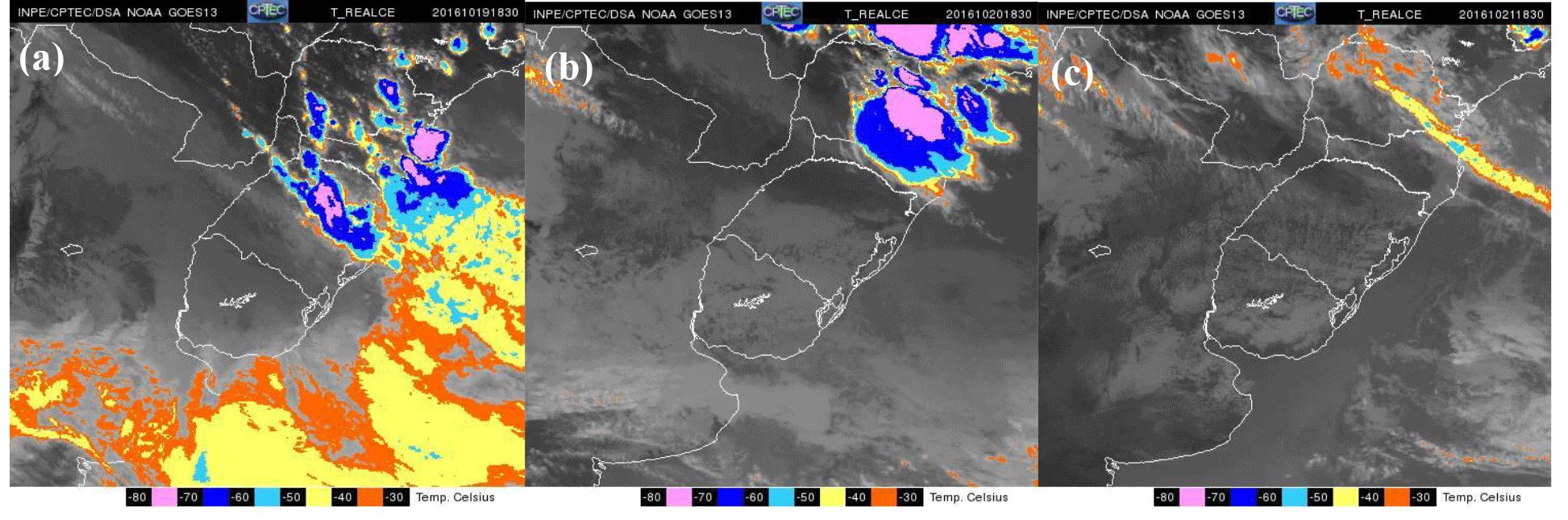
Figure 8Satellite images of GOES 13 for the thermal infrared channel at 18:30 UTC showing the passage of the frontal system over the region on 19 October. The performance of the post-frontal high pressure system without significant cloudiness on 20 and 21 October.
2.3 Tropospheric analysis
After identifying the event, it was the aim that the tropospheric fields show how the troposphere behaved before, during, and after the secondary effect event of the Antarctic ozone hole identified in southern Brazil. The pressure fields at sea level and the layer thickness between 1000 and 500 hPa were obtained to verify which synoptic systems were acting during the event. The presence of the jet is intended to be shown in the field of horizontal winds at 250 hPa and omega values at 500 hPa. In addition, we identified the ascending and descending motions on the surface. Another field analyzed was the vertical cut of the atmosphere at different levels of potential temperature (in Kelvin) and wind (in m s−1) for the longitude of 5∘ W. In this case, the jet current is present in higher levels of the troposphere, which assists in changes of air from the stratosphere to the troposphere.
The Antarctic ozone hole directly influences the Antarctic region where its levels can reach values below 220 DU according to Hofmann et al. (1997). On the other hand, the region highlighted in this study (southern Brazil and Uruguay, at average latitude) suffered indirectly because of this phenomenon. The ozone total column reached a minimum value on 20 October, revealing a possible influence of the Antarctic ozone hole over southern Brazil, as observed in Fig. 1. The event reached southern Brazil on 20 October 2016 (Fig. 1), when the minimum value obtained by the ground-based instrument (Brewer Spectrophotometer) was 225.5 DU (Dobson units), which shows approximately 23 % of reduction in ozone content in relation to climatology data for the month analyzed. On 21 October, ozone-poor air mass remained in the study region, although with less intensity, registering 233.0 DU with a reduction of 19.8 % in relation to the climatology data for the month analyzed. This decrease in ozone content on 20 and 21 October with a slight recovery can be observed in Fig. 1. The black line at 291 DU represents the value of the climatological average for October, where during approximately the whole month the content remained with values below the climatological average. This event was identified as one of the largest ever recorded in southern Brazil, which was similar to the first event observed in the region by Kirchhoff et al. (1996).
Stratospheric dynamic analysis from 19 to 21 October indicates the advance of an ozone-poor polar air mass in southern Brazil at different potential temperature levels (Fig. 2). APV analysis for the three potential temperature levels used in this study can be seen in Fig. 2: 530 K (panels a, b, and c), 600 K (panels d, e, and f), and 700 K (panels g, h, and i). Here, the use of APV at potential temperature levels is due to its ability to function as a dynamic tracer of large-scale air masses, keeping the potential temperature constant (Hoskins et al., 1985). These stratospheric fields show the polar origin of the air mass mainly due to the APV increase from 19 to 21 October in the region of interest (black triangle), thus confirming the occurrence of the event in southern Brazil. Due to its intensity, the air mass persisted in the regions of analysis on 21 October, where the minimum registered ozone content was 233.0 DU, which represents a reduction of ∼ 19.8 %. In addition, the results from the MIMOSA model (Fig. 3) show the direct influence of the ozone hole in southern Brazil at 550 K of potential temperature and approximately 22 km in height. The MIMOSA model retrieved the APV contours shown in Fig. 3 for October 2016 (19, 20, and 21) at 550 K isentropic level (Fig. 3). Because of the change of the APV sign from one hemisphere to another, the colors are reversed in the figure panels on the right (Fig. 3b, d, and f), representing the situation over South America. The blue color indicates the extension of polar air masses up to southern Brazil.
Another model of analysis that showed the displacement of the ozone-poor air mass over southern Brazil was the HYSPLIT/NOAA model. It showed the backward trajectory of polar air mass, as observed by Bresciani et al. (2018). The images of the OMI-ERS2 satellite (Fig. 4) also showed the influence of the Antarctic ozone hole in Uruguay and southern Brazil, where the extension of the area of the hole over the study region can be observed in shades of purple and blue. This information confirms the indirect influence of the Antarctic ozone hole on Uruguay and southern Brazil. As a consequence, a temporary decrease in ozone content was caused on the days of the event.
After identifying the occurrence of the Antarctic ozone hole event in southern Brazil and Uruguay through the analysis of stratospheric dynamics, the following step was to identify which synoptic systems and circulation patterns occurred during the this event. For tropospheric dynamics, the pressure field at mean sea level and thickness between 1000 and 500 hPa can be observed in Fig. 5. Areas highlighted in grey represent pressure – the darker the shade of grey, the lower the surface pressure. Dashed lines represent thickness in units of decameters. The passage of a frontal system over the study region can be observed (Fig. 5a) on 19 October. The arrival of a high-pressure system after the frontal one began to stabilize the atmosphere on 20 October, which indicates a downward movement on the surface. This frontal system operated in the region until 20 October (Fig. 5b), where it began to move towards the ocean. This day presented the largest reduction of ozone content since the mass of air reached southern Brazil and Uruguay. Due to the displacement of this frontal system to the ocean, southern Brazil was under the influence of a post-frontal high-pressure system stabilizing the atmosphere. For 21 and 22 October (Fig. 5c and d), the region was still under the influence of this high-pressure system, where the mass of ozone-poor air that had already reached the region on 20 October day persisted.
After analysis, tropospheric pressure fields were observed at mean sea level, thickness between 1000 and 500 hPa, horizontal cut at higher atmospheric levels, wind at 250 hPa and omega values at 500 hPa, jet stream (grey scale in m s−1), and vertical movement (omega values, solid and dotted lines); see Fig. 6. These fields show the operation of the subtropical jet stream since 19 October (Fig. 6a). The study region, represented by the yellow triangle, was under the influence of a low-pressure system until 22 October (Fig. 6d), when the frontal system moved to the ocean. The presence of negative omega values at 500 hPa on 19 October also reinforced the performance of the front surface system. On 20 and 21 October (Fig. 6b and c), the scenario changed as the subtropical jet flow at 250 hPa was still operating in the region, although with negative omega values at 500 hPa positioned near the polar entry region of the subtropical jet stream. Together with the displacement of the frontal system (Fig. 5b and c), this stabilized the atmosphere where downward movement of the air at low levels is observed. The presence of negative omega values at 500 hPa on 19 October also reinforced frontal surface system performance. On 22 October, we observed a total displacement of the frontal system and the subtropical jet stream to the ocean on the pressure fields at medium sea level and thickness between 1000 and 500 hPa (Fig. 5d) as well as in the fields at high wind levels at 250 hPa and omega values at 500 hPa (Fig. 6d). This way, southern Brazil and Uruguay were under the influence of a high-pressure system on the surface that, along with the positive omega values at 500 hPa, helped stabilize the atmosphere.
The vertical cut of the atmosphere between 1000 and 100 hPa can be observed in Fig. 7. The objective of this field is to analyze the presence of the subtropical jet stream through isentropic levels of potential temperature. The shaded area refers to the presence of the jet stream at high levels. The highlighted black line is the Kelvin potential temperature isolines. The presence of the subtropical jet stream was present on 19 October (Fig. 7a) and 20 October (Fig. 7b), where the lowest concentration value of ozone was recorded for the study region. Additionally, the advance of the jet stream into the ocean can be observed on 21 October (Fig. 7c). For 20 and 21 October, it can be observed near 30∘ S, which indicates a frontal ramp where there is air intrusion from the stratosphere to the troposphere. The high-level fields (Fig. 6) showed the presence of subtropical jet flow at 250 hPa, which, combined with positive omega values at 500 hPa, intensified downward movements and transport of air from the stratosphere to the troposphere (Sthoel et al., 2003). The vertical fields (Fig. 7) for the days of analysis showed the presence of the jet stream at high levels, reaffirming the importance of this circulation for the vertical transport of chemical components such as ozone (Bukin et al., 2011).
The images of thermal infrared channel via GOES 13 satellite at 18:30 UTC (Fig. 8, in blue and pink shades) showed cloudiness on 19 October (Fig. 8a) advancing over southern Brazil to the ocean. For 20 and 21 October, the presence of a high surface pressure system (Fig. 4), together with the presence of the subtropical jet stream at 250 hPa (Fig. 5) and positive omega values at 500 hPa (Fig. 6), favored air stability, leaving southern Brazil and Uruguay without any significant cloudiness.
Tropospheric dynamics showed that the study region was under influence of a frontal system days before the arrival of the mass of ozone-deficient air in the region of Uruguay and southern Brazil. At the surface, the presence of a high-pressure system favored atmospheric stability, where the presence of the subtropical jet stream at 250 hPa, along with positive omega values at 500 hPa, helped explain this intrusion of low ozone air from the stratosphere to the troposphere. Therefore, tropospheric conditions also have a strong influence on the ozone content over midlatitude regions since the jet stream acts as the main tropospheric circulation pattern responsible for transporting stratospheric ozone, playing an important role in the vertical distribution of ozone.
The results obtained in this study show that the methodology used (combined ECMWF reanalysis data and stratospheric and tropospheric dynamics analyses) confirms the occurrence of an extreme event of influence of the Antarctic ozone hole on Uruguay and southern Brazil. The data of the total ozone column showed an intense reduction of its content, especially between 20 and 21 October 2016, where an increase in the potential vorticity was detected at three different levels of potential temperature. In addition, results obtained through MIMOSA also showed an increase in APV over the study region.
In the troposphere, the event occurred after the passage of a frontal system over southern Brazil and Uruguay, where the presence of the jet stream at higher levels helped explain the exchange of air from the stratosphere to the troposphere. For future studies, the objective is to show how often these events occur after the passage of frontal systems as well as to show the subtropical or polar jet stream that most influences the exchange of air masses between the stratosphere and the troposphere during the occurrence of events of ozone depletion.
Ozone surface data (Brewer Spectrophotometer) are not available on international networks. For further information, contact the corresponding author, or send an email to José Valentin Bageston (jose.bageston@inpe.br). Satellite data are available online at OMI-ERS2/NASA (2017). Weather data (ECMWF/ERA-Interim, 2017) are available online after registering at http://apps.ecmwf.int/datasets/data/interim-full-daily/levtype=sfc/. The CPTEC/INPE satellite images are available online at http://satelite.cptec.inpe.br/acervo/goes16.formulario.logic (CPTEC/INPE, 2017).
The authors declare that they have no conflict of interest.
This article is part of the special issue “Space weather connections to near-Earth space and the atmosphere”. It is a result of the 6∘ Simpósio Brasileiro de Geofísica Espacial e Aeronomia (SBGEA), Jataí, Brazil, 26–30 September 2016.
This work is part of the Graduate Program in Meteorology of the Federal
University of Santa Maria (UFSM) in cooperation with the Regional Space
Center Research (CRS) and National Institute of Space Research (MCTIC/INPE),
supported by the Coordination of Improvement of Higher Education Personnel
(CAPES). The authors would like to express their thanks to CAPES/COFECUB
Program, process no. 88887.130176/2017-01, and National Institute of
Antarctic Science and Technology for Environmental Research, CNPq process
no. 574018/2008-5 and FAPERJ process no. E-16/170.023/2008, for the financial
support. The authors also thank NASA for the OMI data, CPTEC/INPE for
satellite images, and ECMWF/ERA-Interim for daily average data.
The topical editor,
Ricardo Arlen Buriti, thanks two anonymous referees for help in evaluating
this paper.
Bencherif, H., Portafaix, T., Baray, J. L., Morel, B., Baldy, S., Leveau, J., Hauchecorne, A., Keckhut, P., Moorgawa, A., Michaelis, M. M., and Diab, R.: Lidar observations of lower stratospheric aerosols over South Africa linked to large scale transport across the southern subtropical barrier, J. Atmos. Sol.-Terr. Phys., 65, 2003.
Bencherif, H., El Amraoui, L., Semane, N., Massart, Charyulu, D. V., Hauchecorne, A., and Peuch, V. H.: Examination of the 2002 major warming in the southern hemisphere using ground-based and Odin/SMR assimilated data: stratospheric ozone distributions and tropic/mid-latitude exchange, Can. J. Phys., 85, 1287–1300, 2007.
Bresciani, C., Bittencourt, D. G., Bageston, V. J., Pinheiro, K. D., Bencherif, H., Schuch, J. N., Leme, N. P., and Peres, V. L.: Report of a Large Depletion in the Ozone Layer over the South Brazil and Uruguay by Using Multi – Instrumental Data, Ann. Geophys., in review, 2018.
Brewer, A. W.: Evidence for a world circulation provided by the measurements of helium and water vapor distribution in the stratosphere, Q. J. Roy. Meteor. Soc., 75, 351–363, 1949.
Bukin, O. A., Suan An, N., Pavlov, A. N., Stolyarchuk, S. Y., and Shmirko, K. A.: Effect that Jet Streams Have on the Vertical Ozone Distribution and Characteristics of Tropopause Inversion Layer, Izvestiya Atmospheric and Oceanic Physics, 47, 610–618, 2011.
Casiccia, C., Zamorano, F., and Hernandez, A.: Erythemal irradiance at the Magellan's region and Antarctic ozone hole 1999–2005, Atmosfera, 21, 1–12, 2008.
Chubachi, S.: Preliminary result of ozone observations at Syowa Station from February, 1982 to January, 1983, Mem. Natl. Inst. Polar Res. Jpn. Spec., 34, 13–20, 1984.
CPTEC/INPE: Division of Satellites and Environmental Systems, available at: http://satelite.cptec.inpe.br/acervo/goes.formulario.logic?i=br, last access: 8 October 2017.
Dee, D. P., Uppala, S. M., Simmons, A. J., Berrisford, P., Poli, P., Kobayashi, S., Andrae, U., Balmaseda, M. A., Balsamo, G., Bauer, P., Bechtold, P., Van De Berg, L., Bidlot, J., Bormann, N., Delsol, C., Dragani, R., and Fuentes, M.: The ERA-Interim reanalysis: configuration and performance of the data assimilation system, Q. J. Roy. Meteor. Soc., 137, 553–597, https://doi.org/10.1002/qj.828, 2011.
Dobson, G. M. B.: Forty years' research on atmospheric ozone at Oxford: A history, Appl. Opt., 7, 387–405, 1968.
ECMWF/ERA-Interim: Daily, http://apps.ecmwf.int/datasets/data/interim-full-daily/levtype=sfc, last access: 16 May 2017.
Farman, J. C., Gardiner, B. G., and Shanklin, J. D.: Large losses of total ozone in Antarctica reveal seasonal ClOx ∕ NOx interaction, Nature, 315, 207–210, 1985.
Gettelman, A., Hoor, P., Pan, L. L., Randel, W. J., Hegglin, M. I., and Birner, T.: The Extratropical Upper Troposphere and Lower Stratosphere, Rev. Geophys., 49, RG3003, https://doi.org/10.1029/2011RG000355, 2011.
Hauchecorne, A., Godin, S., Marchand, M., Heese, B., and Souprayen, C.: Quantification of the transport of chemical constituents from the polar vortex to midlatitudes in the lower stratosphere using the high-resolution advection model MIMOSA and effective diffusivity, J. Geophys. Res., 107, 8289, https://doi.org/10.1029/2001JD000491, 2002.
Hofmann, D. J., Oltmans, S. J., Harris, J. M., Johnson, B. J., and Lathrop, J. A.: Ten years of ozone sonde measurements at the South Pole: Implications for recovery of springtime Antarctic ozone, J. Geophys. Res.-Atmos., 102, 8931–8943, 1997.
Hoskins, B. J., Mcintyre, M. E., and Robertson, A. W.: On the use and significance of isentropic potential vorticity maps, Q. J. Roy. Meteor. Soc., 111, 877–946, 1985.
Kirchhoff, V. W. J. H., Schuch, N. J., Pinheiro, D. K., and Harris, J. M.: Evidence for an ozone hole perturbation at 30∘ south, Atmos. Environ., 33, 1481–1488, 1996.
London, J.: Observed distribution of atmospheric ozone and its variations, in: ozone in the free atmosphere, edited by: Whitten, R. C. and Prasad, S. S., New York, Van Nostrand Reinhold, Chapt. 1, 11–80, 1985.
Marchand, M., Bekki, S., Pazmino, A., LefÈVre, F.,Godin-Beekmann, S., and Hauchecorne, A.: Model simulations of the impact of the 2002 Antarctic ozone hole on midlatitudes, J. Atmos. Sci., 62, 871–884, 2005.
Ohring, G., Bojkov, R. D., Bolle, H. J., Hudson, R. D., and Volkert, H.: Radiation and Ozone: Catalysts for Advancing International Atmospheric Science Programs for over half a century, Sp. Res. Today, 177 pp., 2010.
OMI-ERS2/NASA: Ozone Multi-mission ozone measurements, https://ozoneaq.gsfc.nasa.gov/data/ozone/, last access: 8 October 2017.
OMI-ERS2/NASA: AURA Validation Data Center, https://avdc.gsfc.nasa.gov/index.php?site=1593048672&id=28, last acces: 23 March 2017.
Orsolini, Y. G.: On the formation of ozone laminate at the edge of the Arctic polar vortex, Q. J. Roy. Meteor. Soc., 121, 1923–1941, 1995.
Peres, L. V., Bencherif, H., Mbatha, N., Schuch, A.P., Toihir, A. M., BÈGue, N., Portafaix, T., Anabor, V., Pinheiro, D. K, Leme, N. M.P., Bageston, J. V., and Schuch, N. J.: Measurements of the total ozone column using a Brewer spectrophotometer and TOMS and OMI satellite instruments over the Southern Space Observatory in Brazil, Ann. Geophys., 35, 25–37, https://doi.org/10.5194/angeo-35-25-2017, 2017.
Ploeger, F., Konopka, P., Mueller, R., Fueglistaler, S., Schmidt, T., Manners, J. C., Grooss, J. U., Guenther, G., Forster, P. M., and Riese, M.: Horizontal transport affecting trace gas seasonality in the Tropical Tropopause Layer (TTL), J. Geophys. Res.-Atmos., 117, D09303, https://doi.org/10.1002/2013JD020235, 2012.
Reboita, M. S., Gan, M. A., Rocha, R. P., and Ambrizzi, T.: Regimes of precipitation in South America: A Bibliographical Review, Brazilian Journal of Meteorology,, 25, 185–204, 2010.
Rolph, G., Stein, A., and Stunder, B.: Real-time Environmental Applications and Display sYstem: READY, Environ. Model. Softw., 95, 210–228, https://doi.org/10.1016/j.envsoft.2017.06.025, 2017.
Salby, M. L.: Fund, Atmos. Phys. International geophysics series, Academic Press, Vol. 61, 1996.
Schoeberl, M. R.: Reconstruction of the constituent distribution and trends in the Antarctic polar vortex from ER-2 flight observations, J. Geophys. Res., 94, 16815–16845, 1989.
Seinfeld, J. H. and Pandis, S. N.: Atmos. Chem. Phys.: From Air Pollution to Climate Change, 3rd Edn., John Wiley and Sons, Inc., 2016.
Semane, N., Bencherif, H., Morel, B., Hauchecorne, A., and Diab, R. D.: An unusual stratospheric ozone decrease in the Southern Hemisphere subtropics linked to isentropic air-mass transport as observed over Irene (25.5∘ S, 28.1∘ E) in mid-May 2002, Atmos. Chem. Phys., 6, 1927–1936, https://doi.org/10.5194/acp-6-1927-2006, 2006.