LEO observations of ULF waves can only be reliably done and without too much spatial aliasing for the Pc1/Pi1 and Pc2/3 waves. Due to the fast motion through field lines in a LEO orbit, lower-frequency Pc4–5 waves (1–10 MHz) cannot be accurately determined by LEO satellites, their period being longer than the spacecraft transition time through the wave region. Though Pi2 waves have lower frequencies, thanks to their large spatial scales at low latitudes, they have also been detected by LEO satellites (Sutcliffe and Lühr, 2003; Han et al., 2004; Cuturrufo et al., 2015). Two types of Pc3 waves are observed by LEO satellites: intense localized Alfvén-type waves with transverse magnetic disturbance or weak global compression-type waves recorded in the field-aligned component. In this study, we analyze the magnitude of the magnetic field, thus considering the second type of wave.

In particular, we use the low-resolution magnetic field data with a sampling rate of 1 Hz, and hence we had to limit our analysis to the Pc3 class, covering frequencies from 20 MHz (50 s) to 100 MHz (10 s). An electromagnetic wave of higher frequency, e.g., at 200 MHz, would be captured in the low-resolution data by a pulsation with a period of merely 5 data points, making the analysis statistically dubious.

Our method consists of two parts. The first is the construction of a database of daily power spectra, while the second consists of the actual wave detection. For the construction of the database we used the last available version of magnetic data from the vector fluxgate magnetometer (VFM) instrument (version 4.8 for Swarm A and B and versions 4.9 and 4.10 for Swarm C) as well as additional data from the electric field instrument – EFI (version 4). To further enhance our analysis, we also incorporated data from the daily Level 2 products concerning the FAC and IBI (version 2 for both). For details on the definition and derivation of these products, see Park et al. (2013b) and Ritter et al. (2013), respectively.

For every day in the time interval of interest, which spanned the time period from 15 May 2014 to 15 May 2016, we perform the following analysis. First, the magnetic data cdf files corresponding to the day in question are read, along with the files of the previous and next days. Since all spectral methods are plagued by edge effects (Torrence and Compo, 1998), we append the magnetic field time series of the current day, with a few hours long time series from the previous and next days, so that whatever edge effects appear they will affect these additional “margins”, which can then be safely removed from the process, leaving the spectral data of the day under processing free from such issues. From the magnetic time series of the VFM instrument we derive the magnitude of the magnetic field and subtract from it the total field that is predicted, for the same position and moment in time, by the CHAOS-6 model (Finlay et al., 2016). CHAOS-6 is a geomagnetic field model spanning 1999–2016.5, derived from Swarm, CHAMP, Ørsted, and SAC-C satellite magnetic data and ground observatory data. The model uses spatial differences along-track from CHAMP and Swarm and also east–west differences from Swarm (Kotsiaros et al., 2014). To the derived field time series we then apply a Chebyshev type II, zero-phase, high-pass filter with a cutoff frequency of 20 MHz to remove all lower-frequency components from the signal and to place the Pc3 range in the spotlight (Williams and Taylors, 1988).

A series of studies highlighted the significance of applying wavelet analysis, especially its suitability for multi-point, small-scale disturbances, in the investigation of ULF wave events (e.g., Nosé et al., 1998; Balasis et al, 2012; Xu et al., 2013). Using the wavelet method, with the Morlet mother function, we produce the power spectrum of the magnetic field series for 50 logarithmically spaced frequencies from 20 to 100 MHz (Balasis et al., 2013), and remove the aforementioned margins. In parallel to that, the positional vector of the spacecraft is extracted from the files and converted to magnetic coordinates (magnetic latitude, longitude and local time), as well as the electron density series from the EFI data files of the same day. The final spectrum, along with the time series of the magnetic field, the electron density, and all positional information are then exported in a daily file and saved in the database.

The wave detection begins by reading the daily output files and segmenting them in tracks (half-orbits) from −90^∘ to +90^∘ at magnetic latitude. For each such track, the maximum power per second that is stored in the spectrum is calculated and all segments of consecutive points (seconds) that exceed a threshold of 0.5 nT² Hz⁻¹ (which roughly corresponds to a pulsation with a minimum amplitude of 0.15 nT) are labeled “candidate events”. Each candidate is tested against a series of criteria that help rule out artificial signals that might result from instrument or telemetry errors. As such, for the candidate event to not be discarded, it must exhibit a duration of at least 2 times its peak period, it must have an amplitude that does not exceed certain limits (10 nT), and it must be smooth enough to constitute a continuous pulsation, so its difference series must always be smaller than ±1 nT. These threshold values have been deduced empirically, by visual examination of a large number of events, and it was found that candidates that exceed these values were polluted by spikes or large discontinuities and thus should be removed from the process. In order to avoid traces of activity from lower Pc classes (below 20 MHz) that have not been completely eradicated by the filtering process, we further demand that the peak of the wave activity be at a frequency that does not lie at the limits of the examined range, so only pulsations with a peak frequency that lies above 21 MHz are accepted.

In order to remove events that are influenced or caused by ESFs at low latitudes, field-aligned or auroral currents at higher latitudes, or in general by other, unclassified anomalies in the electron density profiles, we introduce the Plasma Instabilities category and assign to it all wave-like events that can be attributed to these kinds of phenomena. In order to do so, we impose two criteria on the Level 2 product series and demand that in order for a candidate to be a true Pc3 wave event, it must exhibit a value of bubble probability (as defined in the IBI product) of less than 1 % and a field-aligned current amplitude (taken from the FAC product) that is less than 0.5 µA m⁻², both of which must be met for the entire duration of the event. Additionally, if the candidate was detected when the satellite was located in the nightside sector, an additional criterion must be met, namely that its electron density series (extracted from the EFI data files) must not display abrupt changes. In any of these cases the candidate is classified as belonging to the Plasma Instabilities class and is saved in a separate database. On the other hand, if the candidate successfully passes the two criteria for ESF and FAC detection and is located either in the dayside sector or on the nightside, but exhibits a smooth enough electron density series, then it is classified as a Pc3 wave.

In both cases, for every event several characteristics are extracted, such as its duration, peak frequency, average and total power, and bandwidth (the range of frequencies for which the event exhibits power above 50 % of its peak value). All these are saved in a separate matrix for further post-processing and derivation of statistics. For the production of wavemaps, a slightly different approach was used, since waves are by nature extended in space and cannot be accurately represented by a single number (or set of numbers). For this case, the coordinate space, either geographical latitude versus longitude or magnetic latitude versus magnetic local time (MLT), is divided into a 50 by 50 grid, which provides a resolution of 3.6^∘ in latitude, 7.2^∘ in longitude, and slightly less than half an hour in local time. For every second in the duration of an event, its total Pc3 power is calculated and added to the appropriate grid point to which the measurement belongs, based on the satellite's location at the same moment, thus allowing the entire extent of the wave to be accurately represented. In order to make the resulting maps less dependent on the satellite's orbit, we divide the summed power by the number of seconds the satellite has spent in the corresponding point.

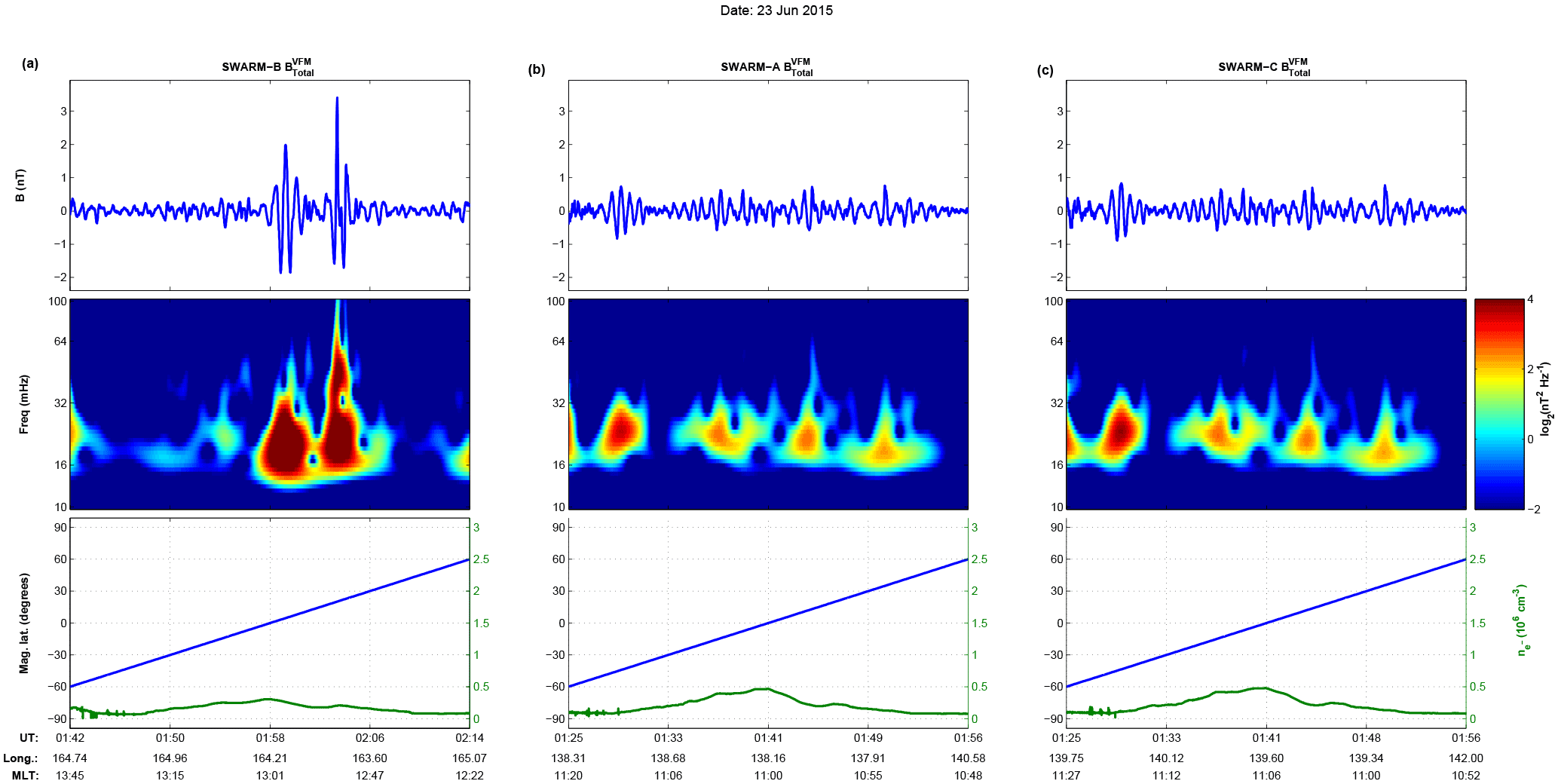
Figure 1Swarm Pc3 wave event. A wave event as detected by the Swarm constellation with Swarm B (a), A (b), and C (c) showing the filtered series of the magnetic field magnitude (top panels), their corresponding wavelet spectra for the joined Pc3 and Pc4 range (middle panels), and a composite plot of the measured electron density (green line) and their location at magnetic latitude (blue line) from −60^∘ to +60^∘ (bottom panels).

Download

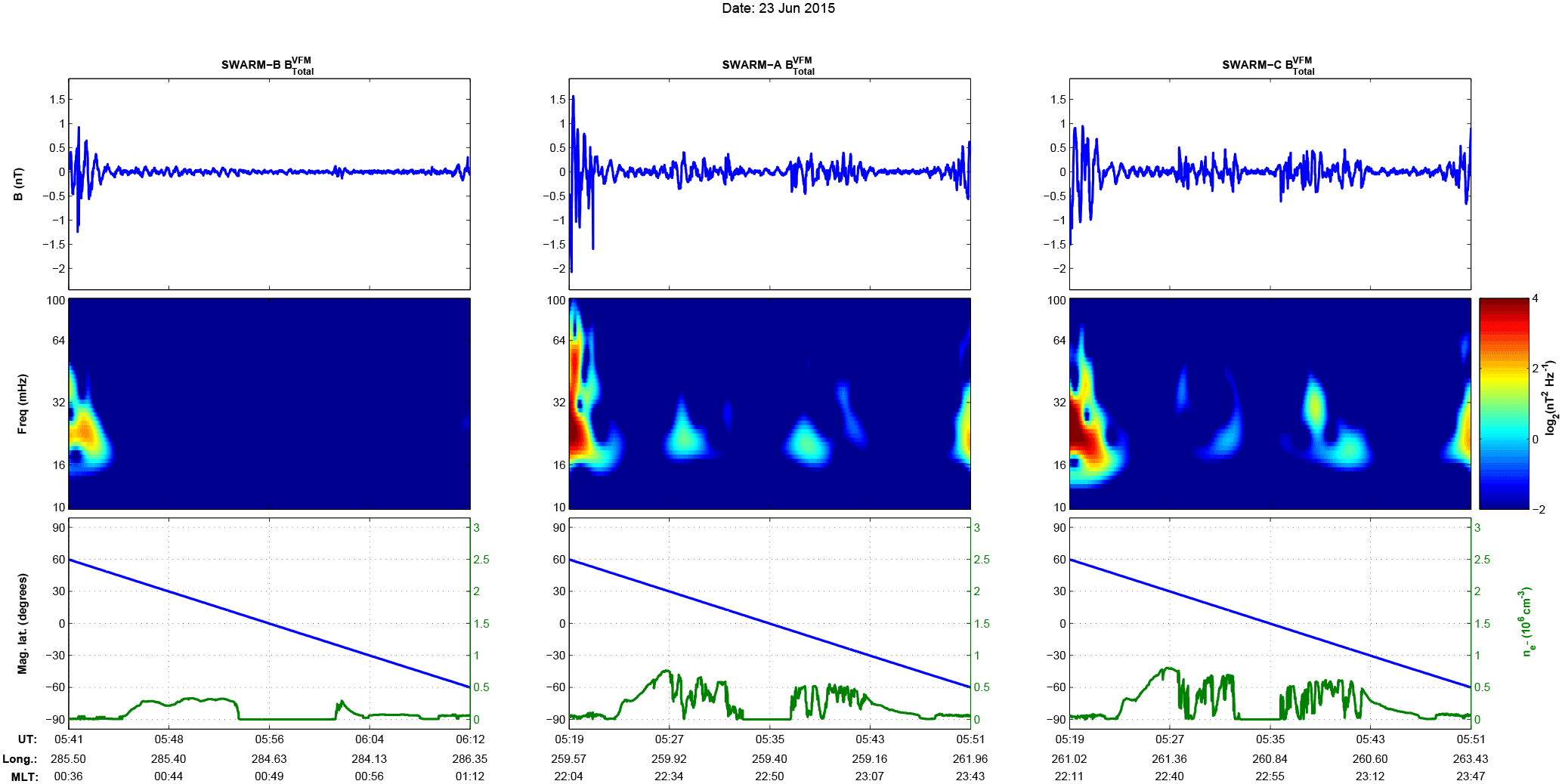
Figure 2Swarm equatorial spread-F event. As in Fig. 1 for another track of the three satellites.

Download

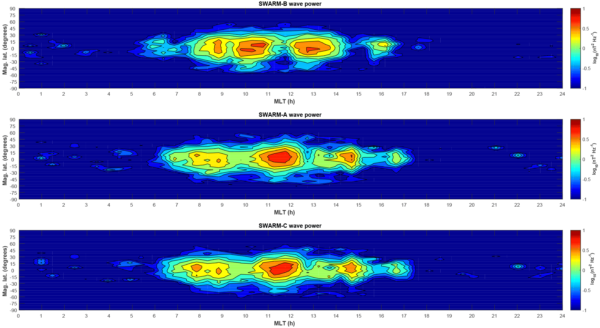
Figure 3Swarm Pc3 wave power map in magnetic coordinates. Pc3 wave power per second mapped on the magnetic latitude versus MLT grid.

Download

Before delving into the wavemaps and the wave index, it is useful to showcase two examples of the methodology applied for our analysis. In Figs. 1 and 2 we show two tracks that correspond to a dayside (MLT ∼ 11:00) detected wave event and a nightside (MLT ∼ 23:00) episode that is attributed to the presence of an ESF event. The data are taken from 23 June 2015, a day which marked the peak activity in the main phase of a geospace magnetic storm, with a minimum Dst index value of −204 nT, at 05:00 UT. The wave event is captured by the northbound pass of all three satellites, here showing only the part from −60^∘ to +60^∘ in magnetic latitude, and is depicted from 01:25 to 01:56 UT for the lower Swarm A and C and, a few minutes later, from 01:42 to 02:14 UT for Swarm B. The ESF-related event is detected only by Swarm A and C on their southbound pass from 05:19 to 05:51 UT and is characterized by the two, symmetric around the magnetic Equator, disturbances in the electron density profile. The ESF events or equatorial plasma bubbles are nightside phenomena identified by their plasma signature as sudden depletions in the electron density profile. We also observe in Fig. 2 the corresponding magnetic signature of the specific ESF event (middle panel), which can be easily mistaken, if it is examined alone, for a wave signature unless the accompanying electron density perturbations are taken into account.

Figure 3 shows the magnetic latitude versus MLT map of wave power for all three satellites of the constellation. As can be seen, the bulk of the Pc3 wave activity is located in the equatorial dayside sector (peaking at 09:00, 10:00–11:00, and 12:00–14:00 MLT for Swarm B and at 08:00–09:00, 11:00–12:00, and 14:00–15:00 MLT for A and C), with the two lower satellites A and C displaying statistically greater power than the higher Swarm B. We note that overall the Pc3 wave activity extends to as early as 06:00 and as late as 17:00 MLT. These results are comparable with the ones derived by Balasis et al. (2015b) for 1 year of Swarm data, with the exception of auroral zones (more information on this issue is given later in this section). The small shift of approximately 2 h in the peaks of the activity between Swarm B and the lower pair is attributed to the angular separation of the orbital planes of the satellites, which for the time period examined ranged from 1 to 2 h in local time. This is a strong indication that all satellites, despite their latitudinal and temporal differences, detect the same events (at least as far as the strongest ones are concerned) and just map them in different local times due to the shift in their orbital planes. As this angular separation increases with time, it will further elucidate the extent in local time of Pc3 wave phenomena. The analogous wavemap in geographic coordinates (latitude versus longitude) is shown in Fig. 4. The striking observation here is that most of the activity is located around the area of the South Atlantic Anomaly (SAA), something that has already been mentioned by Balasis et al. (2015b) and is attributed to the lower magnitude of the geomagnetic field in this region, which favors the occurrence of compressional waves.

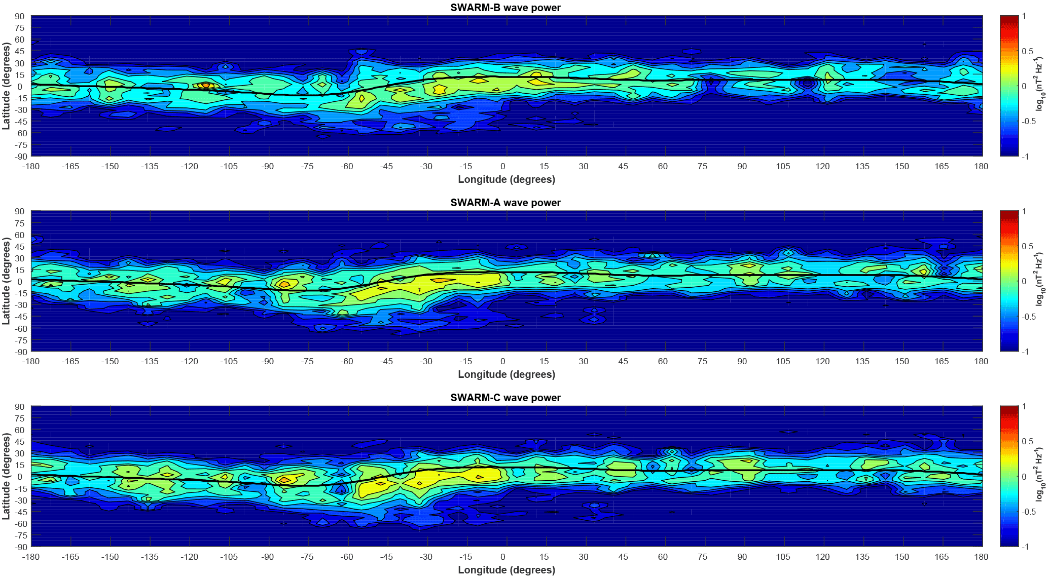
Figure 4Swarm Pc3 wave power map in geographic coordinates. Pc3 wave power per second mapped on the geographic latitude versus geographic longitude grid.

Download

Based on the latitudinal distribution plots of Figs. 3 and 4, there are no Pc3 waves observed at all in the topside ionosphere below −60^∘ or above +60^∘ in both the magnetic and geographic wave power maps, which is obviously an erroneous result. This outcome arises from the application of the Swarm Level 2 single-spacecraft FAC data product correction in our analysis. Since FAC are practically always present at high latitudes, the inclusion of this Swarm Level 2 product apparently eliminates all the Pc3 wave activity there and interprets it as signatures associated with these currents. For this reason, we have finally decided not to use the Swarm FAC product in deriving the final version of the ULF wave power maps based on 2 years of Swarm data, which are now presented in Figs. 5 and 6 in magnetic and geographic coordinates, respectively.

Summing the total power of each detected wave event for every track (half-orbit) and keeping only daytime tracks, we get the total track-by-track power. To reduce the range of these values, which might differ by several orders of magnitude, we define the Pc3 Power Index as the logarithm (base 10) of the total track-by-track power and hence produce the three Swarm Pc3 Power Indices (one for each satellite), which are shown in the top panels of Figs. 7 and 8. Tracks which exhibit index values below 2 are considered “quiet”, while for the rest we can define three different activity levels: “low” for index values between 2 and 3, “moderate” for values between 3 and 4, and “high” for those with index values above 4.

In an attempt to capture the relation between Pc3 waves and geospace conditions, we incorporate into our analysis the time series of various solar wind parameters and geomagnetic activity indices, downloaded from the OMNIWeb Plus data service of NASA's Space Physics Data Facility. These are the magnitude and three Cartesian components of the interplanetary magnetic field (B_IMF) as well as the solar wind velocity (V_sw), both in the GSE coordinate system, the solar wind proton density (N_p), temperature (T_p), the solar wind dynamic pressure (P_dyn), Alfvénic speed (V_Alfvén), sound speed (V_sound) and, based on the latter, the Mach numbers, both Alfvén (M_A) and magnetosonic (M_S). In addition to those we derive the magnetic field's cone angle (θ_B), defined as the angle between the B_IMF vector and its component along the Sun–Earth axis (Greenstadt and Olson, 1976), and the magnetopause standoff distance (R_MP), defined as $R_{\mathrm{MP}}=\mathrm{110.2}(N_{\mathrm{p}}{V}_x^{\mathrm{2}}{)}^{-\mathrm{1}/\mathrm{6}}$ (Kivelson and Russell, 1995). Finally, to incorporate the magnetospheric response to the solar wind, we also include two indices of geomagnetic activity, namely the Auroral Electrojet (AE) index and the symmetric disturbance index for the horizontal component of the Earth's magnetic field (SYM-H). The first, being a high-latitude index, operates as an indicator of substorm activity, while the latter is highly correlated with the disturbance storm time (Dst) index and therefore can be regarded as a proxy for the ring current conditions and thus for geomagnetic storms. All these are depicted in the bottom six panels of Figs. 7 and 8 (for clarity we have ignored the vector components of B_IMF and V_sw and show only their magnitude).

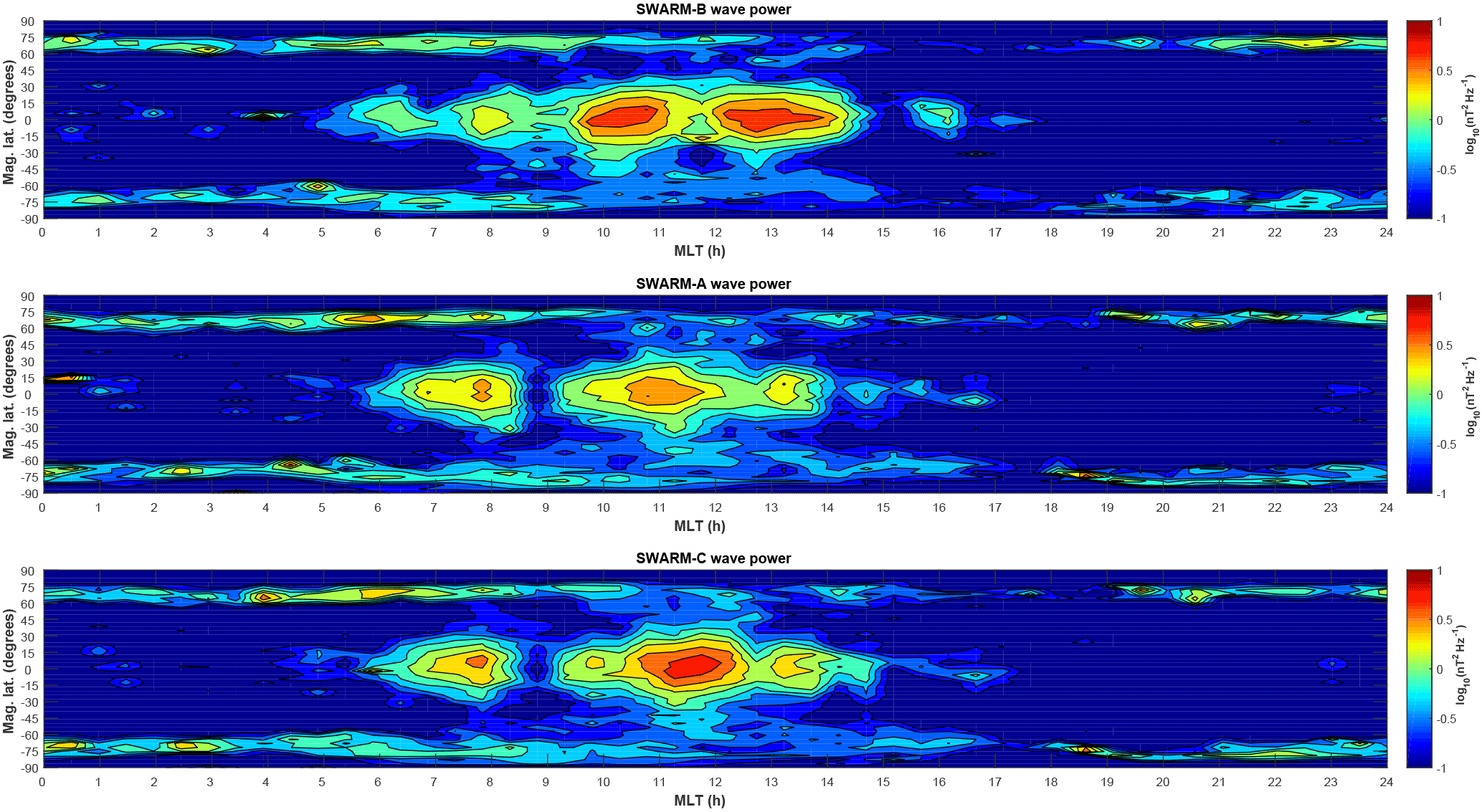
Figure 5Swarm Pc3 wave power map in magnetic coordinates without the FAC correction. As in Fig. 3 without the application of the Swarm Level 2 single-spacecraft FAC data product.

Download

Figure 6Swarm Pc3 wave power map in geographic coordinates without the FAC correction. As in Fig. 4 without the application of the Swarm Level 2 single-spacecraft FAC data product.

Download

Figure 7Swarm ULF wave index time series. From top to bottom: Pc3 power indices for the three satellites of the Swarm constellation (A: first panel, B: second panel, C: third panel), solar wind parameters (V_sw, V_Alfvén, M_A, V_sound, M_S) and the SYM-H index. Ticks on the x axis denote the middle of the corresponding month.

Download

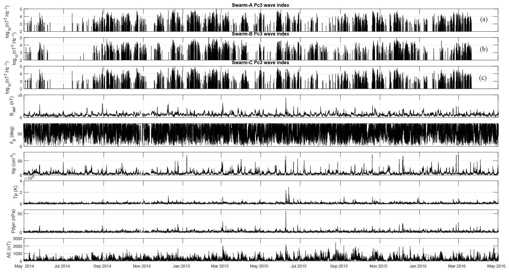
Figure 8Swarm ULF wave index time series. From top to bottom: Pc3 power indices for the three satellites of the Swarm constellation (A: first panel, B: second panel, C: third panel), solar wind parameters (B_IMF, θ_B, N_p, T_p, P_dyn), and the AE index. Ticks on the x axis denote the middle of the corresponding month.

Download

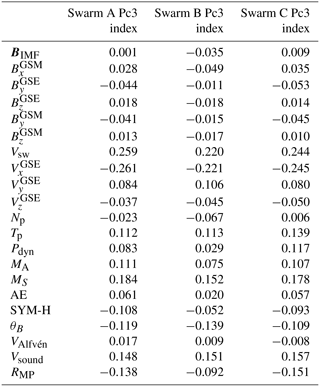
To calculate the correlations between the three Swarm Pc3 Indices and the various solar wind parameters and geomagnetic indices, we considered all possible pairwise combinations, interpolated the parameter series to the timestamps of each Pc3 Index (using a simple, linear interpolation scheme), and computed the Pearson correlation coefficient (Pearson, 1895). The results of this analysis, for all possible combinations, can be seen in Table 1. Looking at the table it becomes evident that the parameter that is most correlated with Pc3 wave activity is the solar wind velocity and especially its component along the X_GSE axis. The negative sign in the V_xGSE correlation just points out the obvious fact that it is the earthward direction that is related to the generation of Pc3 waves. This observation is well known in the literature, as was first made in the 60s (Saito, 1964), but its presence can be seen as a validation of our methodology. Next in order of importance are the magnetosonic Mach number M_S and its corresponding velocity V_sound, along with the magnetopause standoff distance R_MP. For the latter the negative sign indicates that enhanced Pc3 activity takes place when the magnetosphere is most compressed by the solar wind and thus when R_MP exhibits lower values. All these reinforce the idea of Pc3 waves being generated at the bow shock and propagating as compressional mode waves up until the ionosphere, where they are detected by the Swarm satellites (Yumoto et al., 1984; Heilig et al., 2007). Conversely, on the ground these waves are detected as surface geomagnetic pulsations, and thus there the prominent factors are the Alfvénic velocity and its respective Alfvénic Mach number (Heilig et al., 2010), instead of the magnetosonic one which applies to our case. Finally, the last two important parameters are the cone angle, which seems to indicate that enhancements in Pc3 activity are related to low θ_B values and thus to more horizontal B_IMF configurations, and the solar wind's proton temperature T_p. In general though, all correlation values are very low, a fact that is due to the large noise component that characterizes all time series, since for most of the time examined the solar wind parameters exhibit very low (background) levels of activity which are only sparsely interrupted by intense events. We have repeated the analysis using a moving time window with a length that corresponds to 50 tracks, in which case we noticed that for some geomagnetically disturbed periods, the values of the correlations for various parameters can increase dramatically. As an example, for the Pc3 activity at the tail of the August 2014 storm we get correlations with the V_sw that achieve values as high as 0.64 and, for the M_S, values as high as 0.47. Unfortunately, the increase in the correlations does not always follow the increase in geomagnetic activity, so the interplay between these parameters is much more complex and almost certainly governed by nonlinear interactions, although their order of importance remains roughly the same.

As an extra step, we shifted the various parameters' time series by as much as 48 h before and after their actual timestamps, with a time step of 1 h, and re-calculated the correlations, to see whether some specific time lag might yield better results, since the conditions in the solar wind might need several minutes up to a few hours to drive Pc3 waves and allow them to penetrate into the inner magnetosphere until their effects are detected by the Swarm satellites in LEO. Unfortunately this did not yield any meaningful results, since most of the above-mentioned quantities exhibit their peak correlation values for zero time lag and, when they do not, they do not seem to do so in a consistent way for all three satellite indices. The only possible exception is the velocities V_sw and V_sound, which show marginally better correlation factors for a time lag of 2 to 6 h, but the improvements are so small that it is difficult to draw any conclusions from that fact alone.

Table 1Correlation coefficients for each pairwise combination between the three Swarm Pc3 indices and each of the solar wind or geospace parameters for the entire May 2014 to May 2016 period.

Download Print Version | Download XLSX

As for the magnetospheric response to the solar wind, it can be said that the relation between Pc3 waves and magnetic storms is not a simple one. Great storms always coincide with enhancements in Pc3 activity, as can be seen for the January, March, June, October, and December events of 2015, while the extremely quiet period of July and August 2014 also appears completely silent in the wave power series. On the other hand though, significant increases in Pc3 activity do not always coincide with geomagnetic disturbances, as can be seen in the distinct example of February 2015, although for that period there was a moderate increase in V_sw and N_p that consequently led to an increase in M_S. From the two indices employed here, the SYM-H seems to be more correlated with the type of activity that is captured by our Pc3 index, as we mostly focus on equatorial to mid-latitudinal wave activity. The level of the correlations though is again quite low, contrary to the widely spread misbelief that ULF power and geomagnetic activity are closely correlated. This misbelief was refuted recently by Currie and Waters (2014) and it is also evident here, as well.

All data are available through the ESA Earth Online platform, after registration for an ESA Earth Observation Users' Single Sign On account https://earth.esa.int/web/guest/umsso?orig_request=/web/guest/picommunity/myearthnet (ESA, 2018). The AE and SYM-H indices data have been obtained from the World Data Center for Geomagnetism of Kyoto University at http://wdc.kugi.kyoto-u.ac.jp/index.html (WDC, 2018), whereas the solar wind data have been retrieved through the NASA OMNIWeb space physics data facility at http://omniweb.gsfc.nasa.gov/ (GSFC, 2018).

The authors declare that they have no conflict of interest.

This article is part of the special issue “Dynamics and interaction of processes in the Earth and its space environment: the perspective from low Earth orbiting satellites and beyond”. It is not associated with a conference.