The visualization of the mesospheric fronts was made by using airglow images obtained with an all-sky CCD imager (SBIG, STL-1001E model) installed in a shelter close to the Ferraz Station (∼ 1.0 km), but hiding behind a hill in order to avoid the light contamination from the main station. The system uses a near-IR filter with a pass band in the range 715–930 nm, with a notch at 865.5 nm to suppress the O₂ (0–1) emission, to isolate the OH emission with a peak at approximately 87 km altitude (the nominal emission altitude). A telecentric lens is coupled with a high-resolution CCD, 1024 × 1024 pixels, 24.6 × 24.6 mm and ∼ 50 % of quantum efficiency in the near-infrared. The exposure time of the images was 20 s and due to the limitations of the optical system, which was not originally designed for the camera, the images were cropped to 512 × 512 pixels (Bageston, 2011a).

In the calibration process, it is possible to generate four linear projections (km × km) for the unwarped images, that is 256 × 256, 512 × 512, 768 × 768, and 1024 × 1024. For the current analyses, we used the projection of 512 km × 512 km, which gives a resolution of 1.0 km pixel⁻¹ (512 km per 512 pixels), because the wave fronts appeared clearly in this projection.

In order to obtain the parameters of the observed fronts, a two-dimensional FFT (fast Fourier transform) was used, following the methodology described by Wrasse et al. (2007). The methodology consists of selecting a rectangular area in a sequence of 4–5 images; this area must contain the oscillation on all selected images where the front can be seen clearly, without the Milky Way contamination, and this area must contain the wave structure. The horizontal wavelength, observed phase speed, and observed period are obtained from the Fourier spectra.

The wind data were obtained from the meteor radar installed in EACF. The radar consists of eight transmitting Yagi antennas arranged in a circle of 24.4 m, five receiving antennas arranged in an asymmetric cross, and a receiver module. Its operation is on an emission frequency of 36.9 MHz, bandwidth ranging from 35 to 125 kHz, and a power emission peak of 30 kW (Fritts et al., 2012). The radar emits pulses at the above frequencies that are reflected by the trail of gas left by the meteors as they enter in the atmosphere, and this trail is subjected to the local winds. In this way, by the received signal, the radar can measure the wind components in the meteor region, at about 70–110 km height. The methodology behind the estimation of winds is based on a complex correlation adopted to measure the signal phase differences between the receiving antennas in order to determine the echo arrival angle, and complex auto- and cross-correlation methods are used to obtain the rate of change of the relative phase in order to determine the radial velocity associated with the meteor trail, and then the meteor radar provides hourly zonal and meridional winds (John et al., 2011).

Temperature data obtained from the Sounding of the Atmosphere using Broadband Emission Radiometry (SABER) instrument on board the Thermosphere, Ionosphere, Mesosphere, Energetics and Dynamics (TIMED) satellite (Mertens et al., 2001, 2004) were used to calculate the buoyancy frequency (N²) and the squared vertical wave number (m²). The SABER instrument retrieves the temperature in a wide range of altitudes (∼ 15–129 km) based on the non-local thermodynamic equilibrium in the mesosphere and lower thermosphere (MLT) region (Mertens et al., 2009). The TIMED/SABER satellite also provides the volume emission rate (VER) of the OH airglow emission between 60 and 100 km height, which is very important in the present study, mainly in the coincident altitudes of the meteor radar measurements.

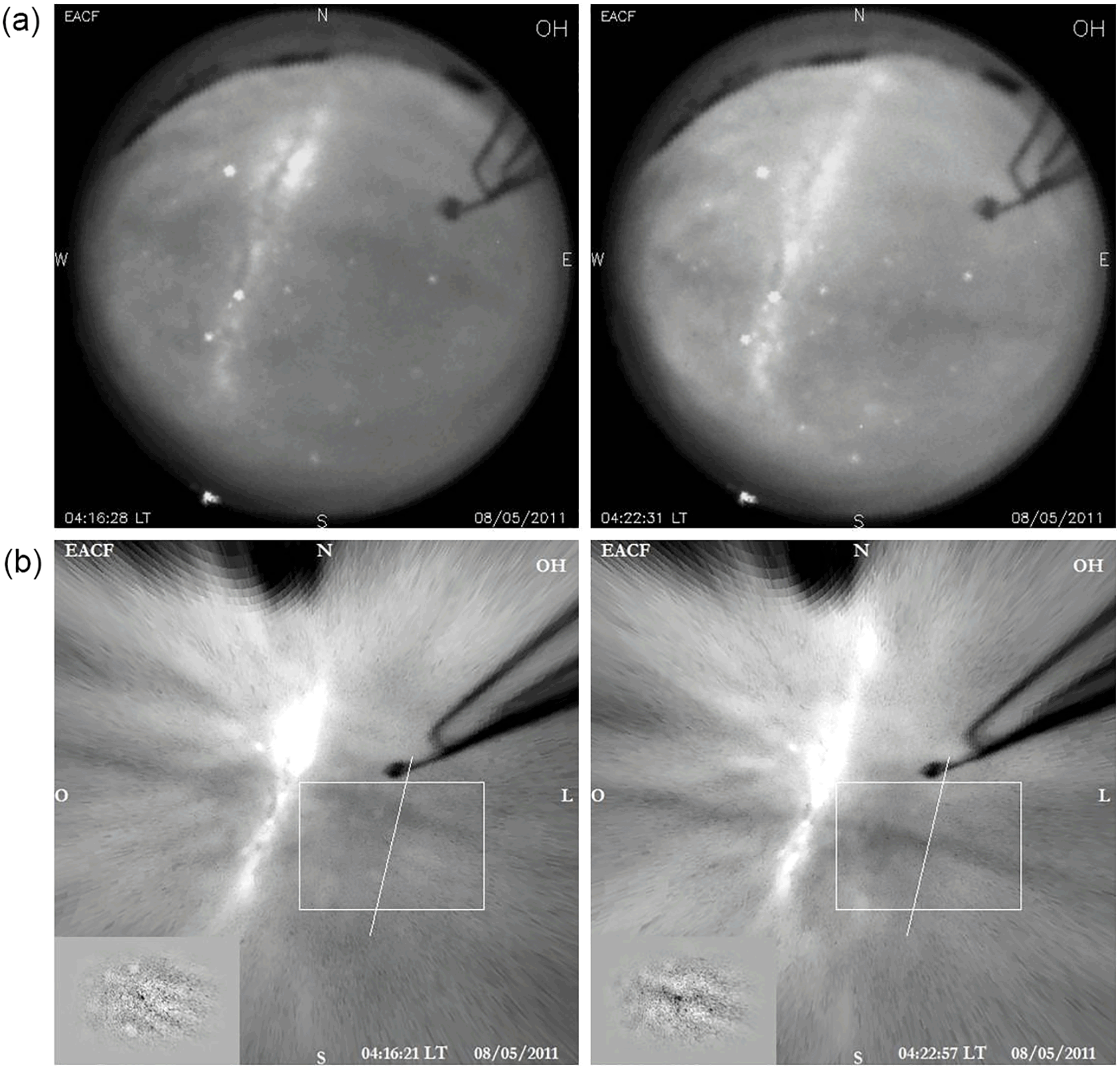
Figure 1Original airglow images (a) and unwarped images (b) used for the spectral analysis of the gravity waves. This mesospheric front was observed on 8 May and characterized with images from 07:15 to 07:23 UT. The lower panels show the images with the star field removed and a small region used for analysis (selected white box), already filtered by a high-pass filter.

Download

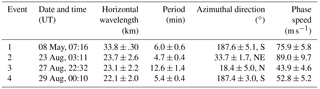
Four mesospheric fronts were observed over the Brazilian Antarctic station during the year 2011. The first event occurred on the night of 7–8 May at 07:16 UT, the second wave front on 22–23 August at 03:21 UT, the third event on 27–28 August at 22:35 UT, and the last reported event was observed on 28–29 August at 00:14 UT.

Figure 1 shows two airglow images for the first frontal event observed in 2011. The first row is the set of two original images and the second row shows the same images but unwarped, where we can see the selected region (white box) in the image for the analysis. The line crossing the box indicates the front propagation direction, while in the bottom left corner the small image is a post-processed (filtered) sub-image used in the spectral analysis. By a visual analysis of the images in Fig. 1, it is possible to identify a wall event propagating south. From the Fourier analysis, the obtained parameters for this event were the following: horizontal wavelength of 33.8 ± 3.0 km, observed period of 6.0 ± 0.6 min, observed phase speed of 75.9 ± 5.8 m s⁻¹, and an azimuthal propagation direction of 193.2 ± 5.1^∘ (southwest). This event appeared in the images at 07:16 UT and about 15 min later it was followed by a large wave structure, in a similar way to recent results presented by Smith et al. (2017); However, in our case it was not possible to associate the possible front generation to this large disturbance structure since we have a weak medium-scale disturbance that occurred nearly orthogonal to the mesospheric front and appeared in the images when the front was already near the zenith.

Figure 2Same as Fig. 1 but for the mesospheric front characterized from 03:11 to 03:16 UT on 23 August.

Download

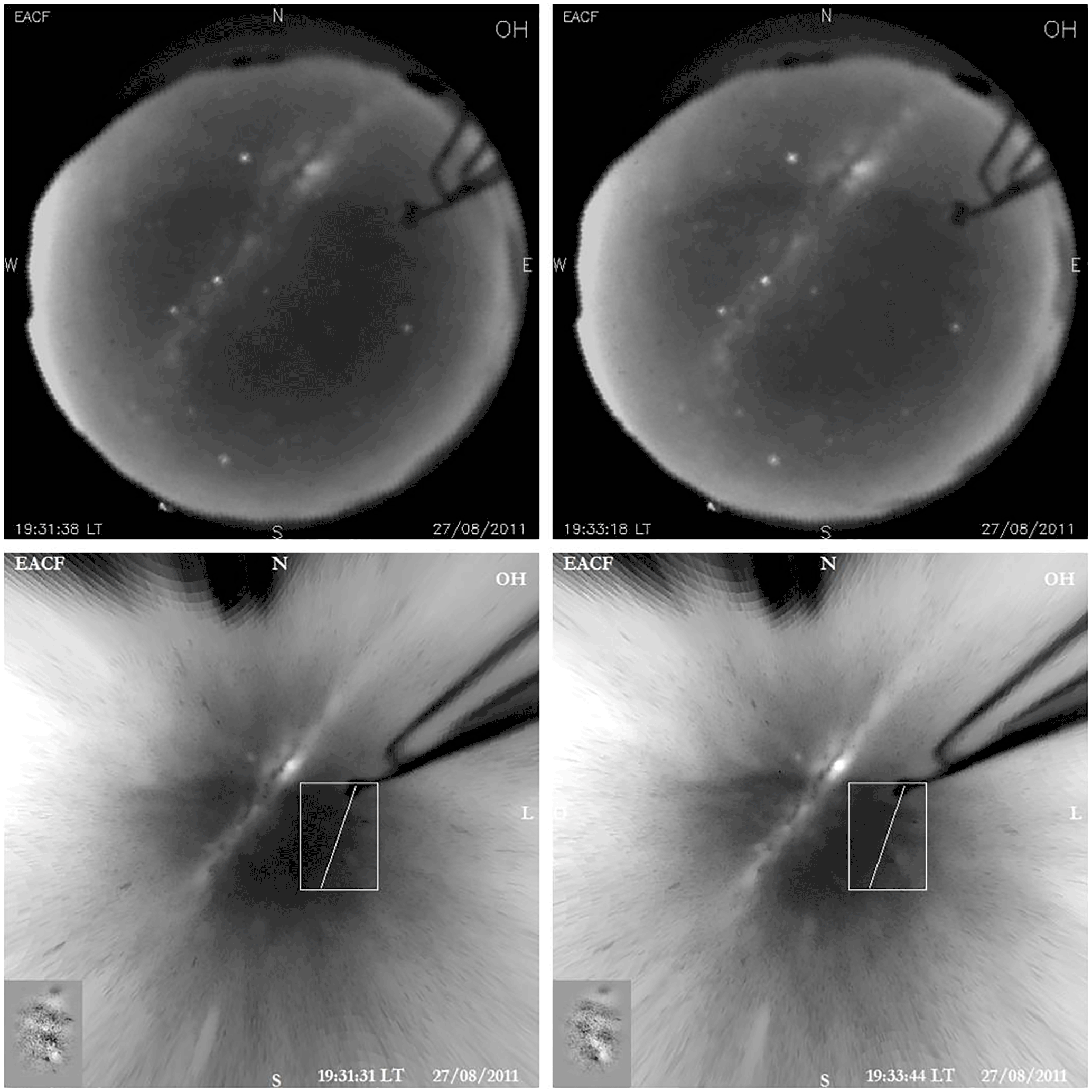
Figure 3Same as Fig. 1 but for the mesospheric front characterized from 22:30 to 22:34 UT on 27 August.

Download

The second event was a front followed by a wave train and an increase in its brightness, and the wave event lasted in the field of view of the all-sky imager for at least 1 hour. However, from 03:30 UT another gravity wave (band type) from the east disturbed the wave train of the mesospheric front, which dissipated during the interaction between the two waves. Figure 2 presents the observation of the second mesospheric front, during the time in which their parameters were analyzed. The first row shows the original airglow images and the second row shows the post-processed images for the spectral analysis. In this case, the obtained parameters, considering the wave train, were the following: wavelength of 23.7 ± 2.6 km, period of 4.7 ± 0.4 min, phase speed of 84.7 ± 5.5 m s⁻¹, and propagation direction of 33.7 ± 1.7^∘ (northeast). Considering only the wave front, it was observed with a phase speed of 89 ± 9.7 m s⁻¹ with a propagation direction nearly to the north.

The third reported event was observed as a dark front followed by a small wave train (not very well defined). Figure 3 shows the observed event in the original images (first row) and it is possible to see the front propagating to the north, followed by small ripples which we can infer to be the wave train. In the second row of Fig. 3, we see the ripples with the box used in order to obtain the wave parameters. The parameters observed for this small wave train were the following: wavelength of 23.1 ± 2.2 km, period of 12.6 ± 1.4 min, phase speed of 30.6 ± 2.9 m s⁻¹, and a propagation direction of 18.4 ± 5.0^∘ (north). For the main front, it was observed with a phase speed of 43.9 ± 4.6 m s⁻¹ and a propagation direction of 356 ± 4.7^∘ (north). The large difference in the propagation direction was due to the location in which the box was placed for the analysis of the front and the wave train. The velocity obtained for this event is quite uncommon, i.e., very low as compared to other typical fronts. This is likely due to the action of the wind decelerating the wave. This will be discussed again in the next section.

Figure 4 shows the last observed event, where the first row shows the original images and the second row presents the respective unwarped images. The analysis for this case resulted in a wavelength of 22.1 ± 2.0 km, period of 5.4 ± 0.4 min, phase speed of 68.4 ± 4.5 m s⁻¹, and a propagation direction of 187.4 ± 3.0^∘ (south). The front presented a phase speed of 52.2 ± 5.2 m s⁻¹ and a propagation direction of 187.6 ± 3.5^∘ (south). All of the parameters for this case and the previous ones are reported as observed parameters. Table 1 summarizes the observed parameter results for the mesospheric fronts described above, together with the fronts identification and date of occurrence.

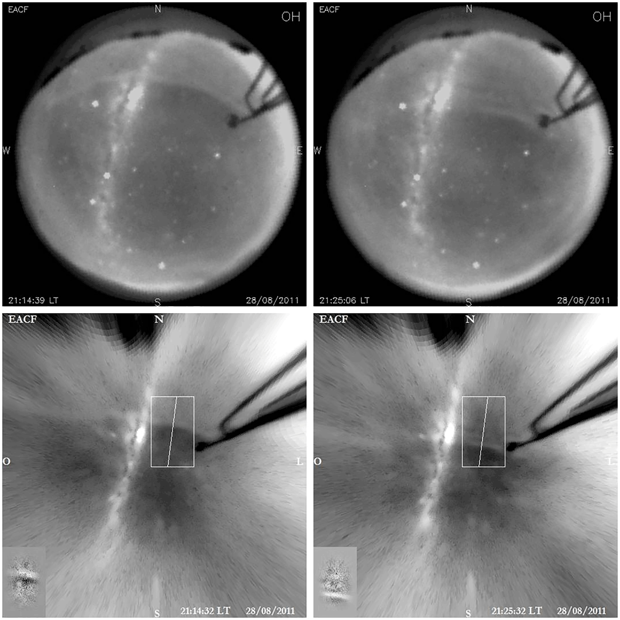
Figure 4Same as Fig. 1 but for the mesospheric front characterized from 00:14 to 00:25 UT 29 August.

Download

We should emphasize that all of the mesospheric fronts showed a step function like the leading fronts. In two cases, the fronts as a minimum of airglow emission (dark fronts) and the other two presented a maximum brightness in the airglow emission. Among the four analyzed cases, only one showed a remarkable wave train, while two of them were basically single fronts (wall-type front) followed by small ripples, and another one appeared as a wide dark region (not too extensive) propagating into a bright region.

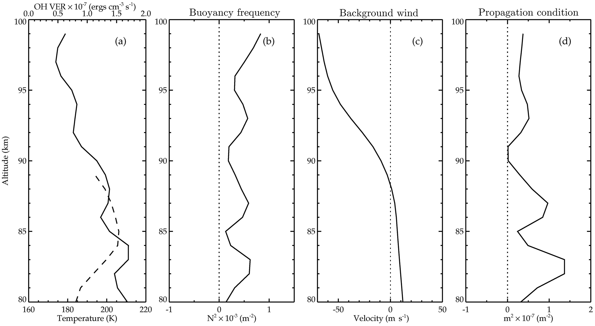
Figure 5Atmospheric profiles for (a) temperature (solid line) and OH volume emission rate (OH-VER, dashed line), (b) buoyancy frequency (N²), (c) wind profile in the wave propagation direction and (d) vertical propagation condition (m²). In this case the profiles were obtained for the mesospheric front observed on 5 May 2011.

Download

Table 1Mesospheric fronts observed in 2011 at Ferraz Station and their respective parameters.

Download Print Version | Download XLSX

Figure 6Same as Fig. 5 but for the mesospheric front observed on 23 August 2011.

Download

In order to characterize the atmospheric duct where these mesospheric fronts propagated, we analyze the vertical propagation condition of each front using the Taylor–Goldstein equation:

In Eq. (1), m² is the vertical wavenumber, u is the wind speed in the wave direction, u^′′ is the second derivative term of the wind speed, c is the observed wave phase speed, k_h is the horizontal wavenumber, and N is the buoyancy frequency, given by the following equation.

In the above equation, g is the acceleration due to gravity, T is the temperature, C_P is the specific heat at constant pressure, and ∇T_Z is the temperature gradient.

Equation (1) is a dispersion relation valid for gravity waves propagating in an environment where the effects of horizontal winds and temperature gradients cannot be neglected (Chimonas and Hines, 1986; Isler et al., 1997; Fritts and Yuan, 1989). The analysis of this equation can provide the wave propagation conditions; that is, if m² > 0, then the wave can freely propagate vertically; if m² < 0, then the wave is not allowed to propagate vertically; and, lastly, in the case where the region of m² > 0 is surrounded by two regions of m² < 0, this interval of m² > 0 is called a ducted region.

Then, based on the Eqs. (1) and (2) and using temperature data from the SABER instrument, and wind data from the meteor radar, one can estimate if the required ducts for the events to propagate exist. In the case of confirmation of favorable conditions for ducted waves, then it is possible to analyze if the duct was due to the temperature structure (thermal duct), basic wind contribution (Doppler duct), or contributions from both temperature and wind (thermal-Doppler duct).

Figure 5 shows the vertical profiles for the atmospheric environment and propagation conditions for the first event, which occurred between 7–8 May. Figure 5a shows the vertical temperature profile (solid line) with the OH volume emission rate (OH-VER; dashed line), using the closest SABER sounding to the EACF, Fig. 5b shows the buoyancy frequency calculated with the temperature shown in Fig. 5a. Figure 5c presents the wind profile in the direction of wave propagation, and finally, Fig. 5d shows the m² propagation condition. For the night of 7–8 May there were just a few SABER soundings near the EACF and the closest sounding was about 4 h before the event occurrence and distant ∼ 300 km from the station. The temperature profile presented in Fig. 5a is an approximation of the thermal environment in the surroundings of the station from where the front was identified, because it is very difficult to obtain simultaneous SABER observations with a rare gravity wave event, especially for Antarctic latitudes. From the OH-VER emission observed by the TIMED/SABER satellite, it is possible to identify the peak height of the OH airglow emission. As can be seen in Fig. 5, the front was confined between about 82 and 90 km height where m² > 0, with the emission peak around 85 km height and a double duct structure in this altitude interval, but with the main duct associated with this wave front between 80 and 85 km. None of the graphs were plotted below 80 km because there was no wind measurements below this height. In this case, we can infer that the approximate duct formation is characterized mainly by the temperature vertical structure (thermal favorable condition), since the m² profile is very similar to the buoyancy frequency and the wind profile did not show significant variation (∼ 10.0 m s⁻¹) from 80 to 89 km height. However, this condition (not a true duct) could maintain the wave front to be quite stable and propagating mainly horizontal, but also vertically (m² > 0).

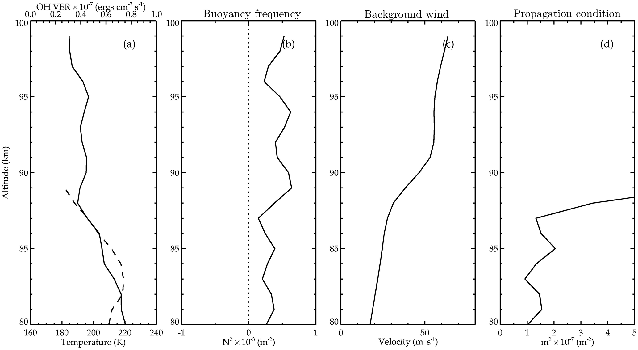
Figure 6 shows the vertical profiles for the atmospheric environment and propagation conditions for the second event, which occurred between 22–23 August. The graphs in Fig. 6 represent the same variables and in the same way as presented in Fig. 5, but now for the parameters of the second wave front. For this day, the closest SABER sounding was obtained approximately 5 h before the observed time of this event and 420 km away from EACF. In Fig. 6a, it is observed that the OH emission layer is located between 81 and 88 km, with the peak at 85 km, so we focus the analysis in this altitude interval, even though the more pronounced m² is located above 90 km height. The temperature is decreasing from 80 to 82 km and then turns to increasing up to 87 km, and this small inversion leads to duct-like in the buoyancy frequency and also in the m² profile in this altitude interval. Again, the propagation condition is similar to the previous case, having no influence by wind conditions in the region of the OH airglow layer. Thus, the duct-like condition for this case was also caused by the temperature.

Figure 7Same as Fig. 5 but for the mesospheric front observed on 27 August 2011.

Download

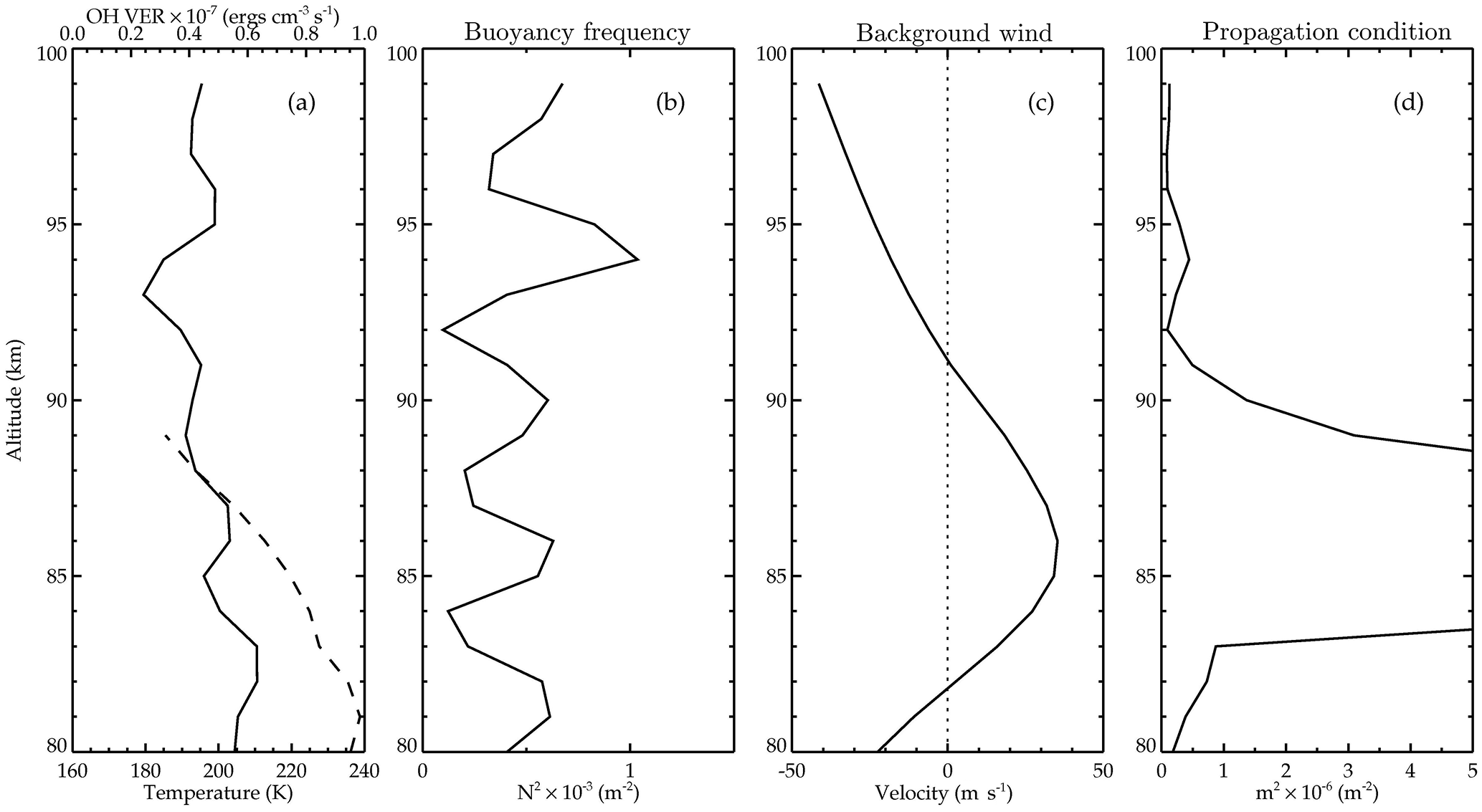
Figure 7 shows the atmospheric background environment and propagation conditions for the third event. In this case, we can see a clear correlation between the background wind and m². A duct is clearly visible centered on 86 km, several km above the OH peak which is located at 81 km. It is noteworthy that the m² is very near to an ideal duct condition, although m² does not become negative below 82 km and above 92 km, because the temperature profile did not contribute to the formation of this ideal duct. It is also noted that two strong inversions in the wind occur at 82 and 91 km height and this wind shear generated the ideal conditions for a Doppler duct. Another interesting aspect for this case is the fact that the wave has a phase speed approximately equal to the wind speed; consequently, the two wind shears that characterize the duct were absorbing the wave energy as the wave was approaching the critical level (Nappo, 2002). The closest temperature profile used was obtained about to 2.5 h before the wave front occurrence and approximately 370 km away from Ferraz Station (inside the field-of-view of the all-sky imager), but this temperature did not influence the formation of the duct.

Figure 8Same as Fig. 5 but for the mesospheric front observed on 29 August 2011.

Download

The environment and propagation conditions for the last event are shown in Fig. 8, in the same format as in the previous figures. The SABER profiles were obtained about 4 h before the occurrence of this wave front, i.e., it is a rough approximation for the temperature at the instant of occurrence of the front and may not represent the thermal structure over the observatory around the time of the wave front observation. The temperature profile within the OH layer presented a small and constant decreasing rate (∼ 3 K km⁻¹), between 81 and 86 km, without significant variability, so did not form a thermal duct configuration, as observed in the N² profile in Fig. 8b. On the other hand, the wind profile along the wave direction (obtained between 00:00 and 01:00 UT), as shown in Fig. 8c, was relatively weak and almost constant between 80 and 88 km height. The wind characteristics coupled with the thermal conditions were not enough to generate a duct configuration, as can be noted in Fig. 8d. In this way, the m² did not present a duct, i.e., the front could be considered to be vertically propagating considering the above observed atmospheric background even knowing that this kind of wave needs a duct structure, which was not observed due to the lack of satellite data close to the time of the wave observation. These conditions coupled to other gravity waves propagating simultaneously, and almost orthogonal, caused a destruction of this wave front around 00:43 UT (see the respective video in the Supplement), just after passing the zenith. We suggest that in this case, the wave structure was absorbed by the local environment and contributed to accelerate the background wind, as observed between 90 and 95 km height in Fig. 8c and also in the Supplement (last slide of the .pdf file), where it is noted at 01:30 UT around 93 km height.

Figure 9Satellite images before the mesospheric observations. The green triangle represents the position of Ferraz Station and the arrows represent the direction of the front propagation. Event 1 occured approximately 5 hours before the observation of the front, Event 2 about 3 hours before the observation, Event 3 about 2 hours before the observation, and Event 4 about 4 hours before the observation. Source: Center for Weather Forecasting and Climate Studies of the National Institute for Space Research (CPTEC/INPE).

Download

At first, it is interesting to note that we have observed four wave front events in the whole year of 2011 but three were observed in a single week at the end of August, which means that some anomalous phenomena would be occurring in the surroundings of the Brazilian Antarctic station (directly in the troposphere or indirectly in the mesosphere). Thus, to investigate the origin of such mesospheric fronts, we analyzed satellite images to look for instabilities or forcing structures, which could generate theses waves. Figure 9 shows four satellite images a few hours before the events observed in the mesosphere. Additionally, an animation (.gif file) for each observed day was added as a Supplement.

The first event is similar to a peculiar wave event reported by Smith et al (2017) who presented a twin bore event that occurred over Europe in March 2013 and their analysis suggested that these bores were associated with a larger-scale mesospheric disturbance, which was associated with a severe meteorological phenomenon (cold front). In our observation, the similarity is based on the fact that we also observed a large-scale disturbance after the front has passed the zenith, just behind the mesospheric front. However, in our observation, the mesospheric disturbance was tenuous and difficult to identify, and was possibly not the proper source of this mesospheric front. On the other hand, 5 h before the front observation, a cyclonic system was present north of Ferraz Station, as can be seen in Fig. 9a. This kind of system is a potential wave source already identified and linked to gravity waves in the mesosphere near the Antarctic Peninsula (Bageston et al., 2018). The cyclones are commonly observed around the peninsula and have been reported by several authors (e.g., Heinemann, 1990; Carrasco et al., 2003). Cyclones can release a large amount of energy into the atmosphere due to the fact that rotational kinetic energy is converted to linear kinetic energy, which in turn generates hydrodynamic instability. This kind of instability is able to generate gravity waves that can propagate up to the mesosphere. Thus, in this first case, we are associating the frontal wave observed in the OH airglow layer to a cyclonic activity in the troposphere, which match very well with the typical time of propagation of the gravity waves from the troposphere to the mesosphere (2 to 6 h) and also because the location of the meteorological system is exactly at the location from where the wave in the mesosphere was observed to come from.

The second mesospheric wave front event is quite similar to the event described by Bageston et al. (2011b) in terms of its morphology, i.e., a remarkable wave front followed by a series of wave crests confined in a very well-defined duct, with the main contribution from the wind structure, but different from the present case, which showed a thermal duct condition for the front propagation. For this case, the potential source in the troposphere is shown in Fig. 9b which presents a large cloud condensate south of Ferraz Station, with a large potential of convective instability as can be seen in the animation (.gif) posted as Supplement, because the clouds near the center of the condensate are very high and much colder (< −70 ^∘C) than the surroundings (−30 to −50 ^∘C) and in the center of this cloud the convection should be very intense. In this case, the potential source in the troposphere was associated with a strong convection generated from the cloud cell identified in Fig. 9b, and a thermal propagation condition (see Fig. 6b and d) in the mesosphere that allowed the wave to propagate from the Antarctic Peninsula to the observatory (Ferraz Station).

For the third event, Fig. 9c shows no evidence of any meteorological phenomena able to generate gravity waves in the troposphere. Also, the dark wave front (a wide depletion airglow region) seen in the all-sky images was not very well defined and we can infer that this observed wave in the mesosphere was generated by a wave–wave interaction or from wave breaking at lower mesospheric heights. As this front was vanishing, it is very likely that such a front was absorbed by the background once the wind was increasing fast in the same direction of the wave propagation (inside the OH layer), as noted in Fig. 7c between 81 and 85 km height, and at some point the wave speed reached the same velocity as the wind. So, for this wave front, the associated source was linked to a dynamical disturbance at mesospheric heights and its dissipation occurred by the wind blowing in the same direction as the wave propagation direction.

The fourth front event was very similar to the third one, but they were propagating in opposite directions. Analogously to the previous case we check the tropospheric situation during the night of the observed event, this is presented in Fig. 9d and it can be noted that no meteorological phenomenon is seen in a radius 1000 km north of the station. Due to the lack of meteorological conditions to support the generation of this event, we can not associate any tropospheric source as a reliable physical mechanism capable of generating the observed wave front. This indicates that other stratospheric or mesospheric phenomena (such as wave breaking or wind shear) should be claimed as the potential wave source, but it is difficult to access such sources since the only available wind data for the troposphere and stratosphere are the meteorological reanalysis.

The occurrence of mesospheric fronts in the Antarctic Peninsula is quite unusual for that geographical region according to previous works (Nielsen et al., 2006; Bageston et al., 2011a, b). However, the present work reports unusual occurrences of mesospheric fronts above Ferraz Station in 2011, and mainly concentrated in a short period of time (1 week). For these three last cases, only one could be associated with meteorological phenomenon and the other two have possible in situ generation. So, the important contribution of this work is not only the report of four mesospheric fronts but also the idea that the main mechanism responsible for wave front generation may not be in the troposphere.

Contact David Fritts (dave@gats-inc.com) for meteor radar measurements over EACF. SABER measurements are available online in the Internet. Airglow images from EACF can be solicited directly by e-mail to José Valentin Bageston (bageston@gmail.com). The CPTEC/INPE satellite images are available online at: http://satelite.cptec.inpe.br/acervo/goes16.formulario.logic (CPTEC/INPE, 2017).

The supplement related to this article is available online at: https://doi.org/10.5194/angeo-36-253-2018-supplement.

The authors declare that they have no conflict of interest.

This article is part of the special issue “Space weather connections to near-Earth space and the atmosphere”. It is a result of the 6^∘ Simpósio Brasileiro de Geofísica Espacial e Aeronomia (SBGEA), Jataí, Brazil, 26–30 September 2016.