The M-transform function is a 3-D FFT function using Interactive Data Language (IDL; http://www.exelisvis.com/ProductsServices/IDL.aspx, last access: 15 September 2018), which is used to analyze airglow imaging data based on the method developed by Matsuda et al. (2014). This method requires time series of airglow images in 3-D array format, which have been preprocessed to have fixed intervals of image pixels (dx, dy) and time (dt). These preprocessed images should be obtained through common airglow image preprocessing, that is, (1) star removal, (2) correction of the Van Rijhin effect if necessary, and (3) projection onto a geographical coordinate system in equal distances in latitudinal and longitudinal directions (e.g., Kubota et al., 2001; Suzuki et al., 2007). It is also recommended to normalize the airglow intensity values to compare the power spectral values of different datasets. For this purpose, ($(I-\stackrel{\mathrm{‾}}{I})/\stackrel{\mathrm{‾}}{I}$), where I is the image intensity of each pixel, should be used in the input array. Our M-transform code applies 2-D prewhitening to the images to reduce the contamination of higher wavenumbers with lower-wavenumber peaks of the red AGW spectrum. It also applies the 2-D Hanning window to reduce the harmonics of the window function in the horizontal direction (Coble et al., 1998). Matsuda et al.'s (2014) new method transforms the power spectrum density (PSD) in the wave number domain (k, l, ω) to the phase velocity domain (ν_x, ν_y, ω) based on the following equations:

where v_x and v_y are the orthogonal projections of the phase velocity onto zonal and meridional axes, respectively ($({\mathit{\nu }}_x,{\mathit{\nu }}_y)=c(\sin \mathit{\phi },\cos \mathit{\phi })$, where c and φ are the phase speed and azimuth (east from north) of the phase velocity). Note that ν_x and ν_y are not the phase velocities in the zonal or meridional directions or cross sections; ω is the frequency; and k and l are the zonal and meridional wavenumbers, respectively. Finally, the phase velocity spectrum is integrated over the frequency and results in a 2-D phase velocity spectrum.

Table 1Description of M-transform function on IDL.

Download Print Version | Download XLSX

The original program developed by Matsuda et al. (2014) consisted of several subroutines, which were used to calculate the 3-D FFT, create an interpolation table, perform the interpolation, and separately plot the results. The users had to set the wave parameters in each subroutine and had to run it one by one, making the process complicated and inefficient. Furthermore, once the users failed to compile one of the subroutines, the program failed to run and the users had to check the subroutine one by one again. Therefore, a simple, hassle-free one-line-command software with adjustable input keywords is necessary to efficiently apply this method.

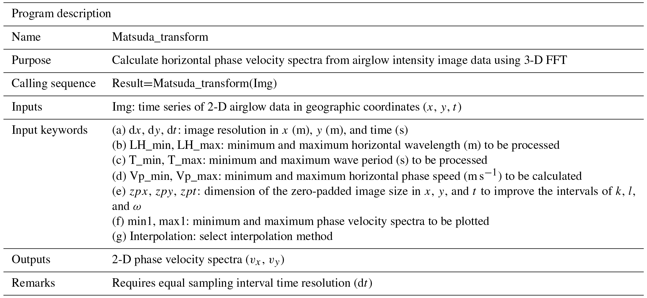
Table 1 shows the description of the M-transform function and Fig. 1 shows how to run the program. To run this function, the user can simply use the calling sequence “Result=Matsuda_transform(Img)”, where “Img” is the 3-D array of the preprocessed images in geographic coordinates (x, y, t). The image resolutions (dx, dy, dt), wave parameters (horizontal wavelength, LH), wave period (T), phase speed (Vp), and size of zero padding (zpx, zpy, zpt) can be adjusted by setting input parameter keywords. The default image resolution is 1 km in both zonal (dx) and meridional (dy) directions. The default image interval time (dt) is 60 s. The default minimum and maximum values of the wave parameters are $\mathrm{5}\le \mathrm{LH}\le \mathrm{100}$ km, $\mathrm{8}\le T\le \mathrm{60}$ min, and $\mathrm{0}\le \mathrm{Vp}\le \mathrm{150}$ m s⁻¹. The default output of this program is a 2-D phase velocity spectrum. The default interpolation method of this new function is the Delaunay triangulation method (e.g., Dwyer, 1987; Su and Scot Drysdale, 1997). One restriction of this program is that it requires an equal time interval (dt). This may not be the case for practical observations, where filter rotations or background (or dark) images for the calibration are obtained from the observation sequence. In that case, users have to interpolate the image to obtain a constant dt interval before applying this function. More details on the function development are provided elsewhere.

Figure 1Flow chart showing the input, how to run the program, and the output format.

Download

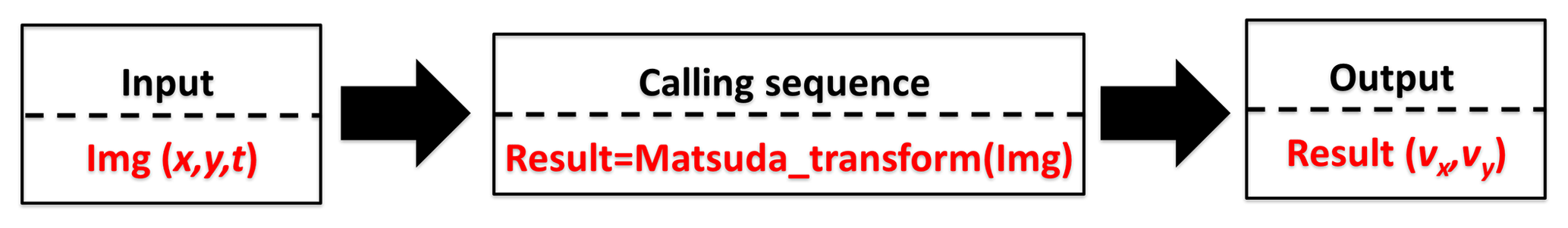
Figure 2 shows an example of the use of the M-transform function. The input consists of airglow data over the Syowa Station obtained on 20 September 2011 (the same dataset as used in Matsuda et al., 2014), which have the following dimensions: x=400 km, y=400 km, t=21 min (×3 min). Because the image time resolution was 3 min, the dt input keyword was set to dt=180 s. The default values were used for the other wave parameters. The IDL console shows the input, calling sequence, total calculation time, and output. The output is a 2-D phase velocity spectrum (right panel). The horizontal axis is v_x, the vertical axis is v_y, and the color bar shows the PSD on a logarithmic scale. The phase velocity spectrum shows dominant propagation in the southwestward direction, which agrees with the wave propagation observed in the airglow preprocessed image movie in the Supplement as that reported by Matsuda et al. (2014). The total calculation time of the M-transform function for 21 images with 400×400 pixels was ∼1.4 min using a personal computer. The calculation was performed on a MacBook Pro with a dual core 2.8 GHz Intel Core i7 processor with 4 MB cache size and 16 GB memory, while the program was single-threaded.

Table 2Summary of airglow imagers used in this study.

Download Print Version | Download XLSX

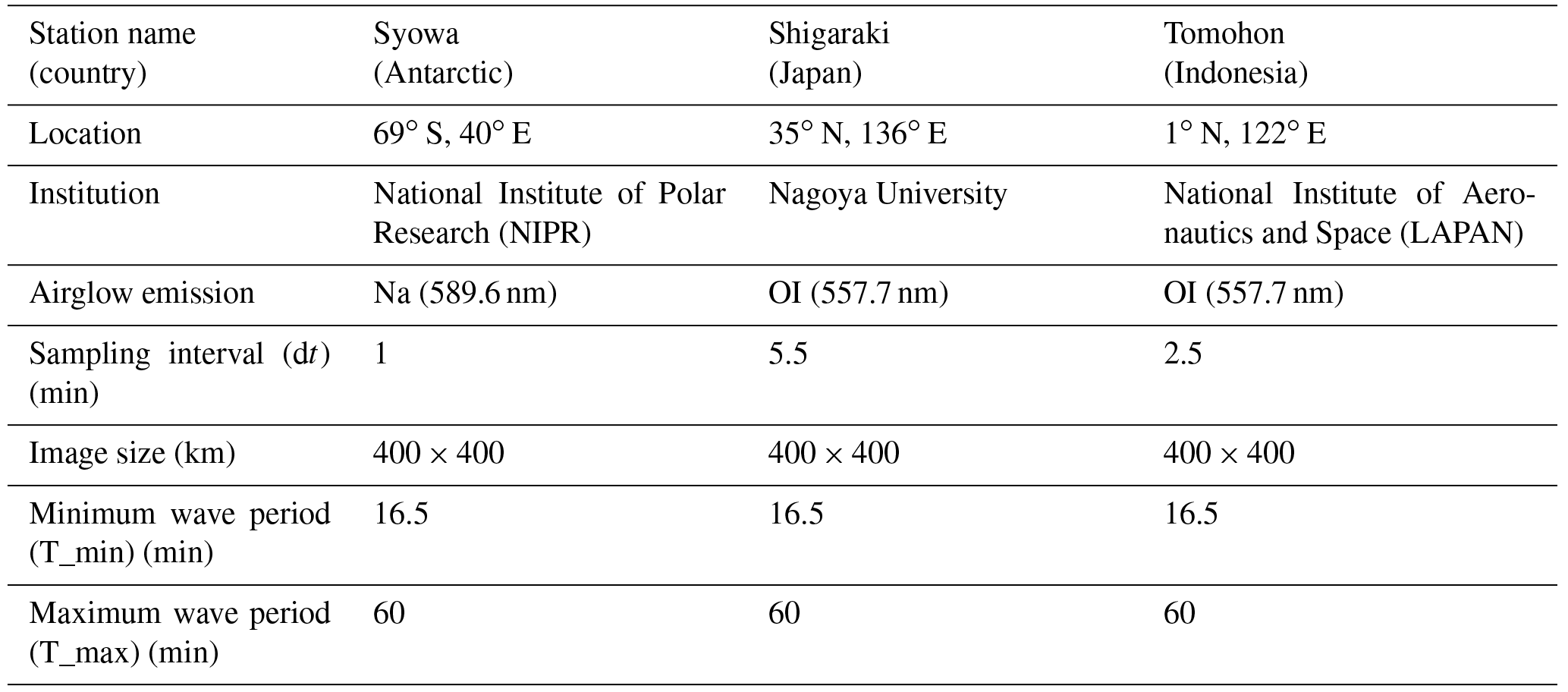
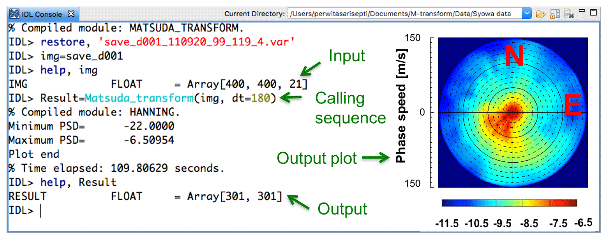
Figure 2Example of how to use the Matsuda-transform (M-transform) program, showing the input, calling sequence, total calculation time, and output as 2-D phase velocity spectrum.

Download

We applied this new M-transform function to various airglow datasets obtained at three different latitudes. Table 2 shows the summary of each airglow imager used in this analysis. Syowa Station (69^∘ S, 40^∘ E) data represent airglow data in the polar region, while Shigaraki (35^∘ N, 136^∘ E) and Tomohon (1^∘ N, 122^∘ E) data represent the midlatitude and equatorial regions, respectively. We used the Na (589.6 nm) airglow emission obtained at the Syowa Station and OI (557.7 nm) airglow emission recorded in Shigaraki and Tomohon.

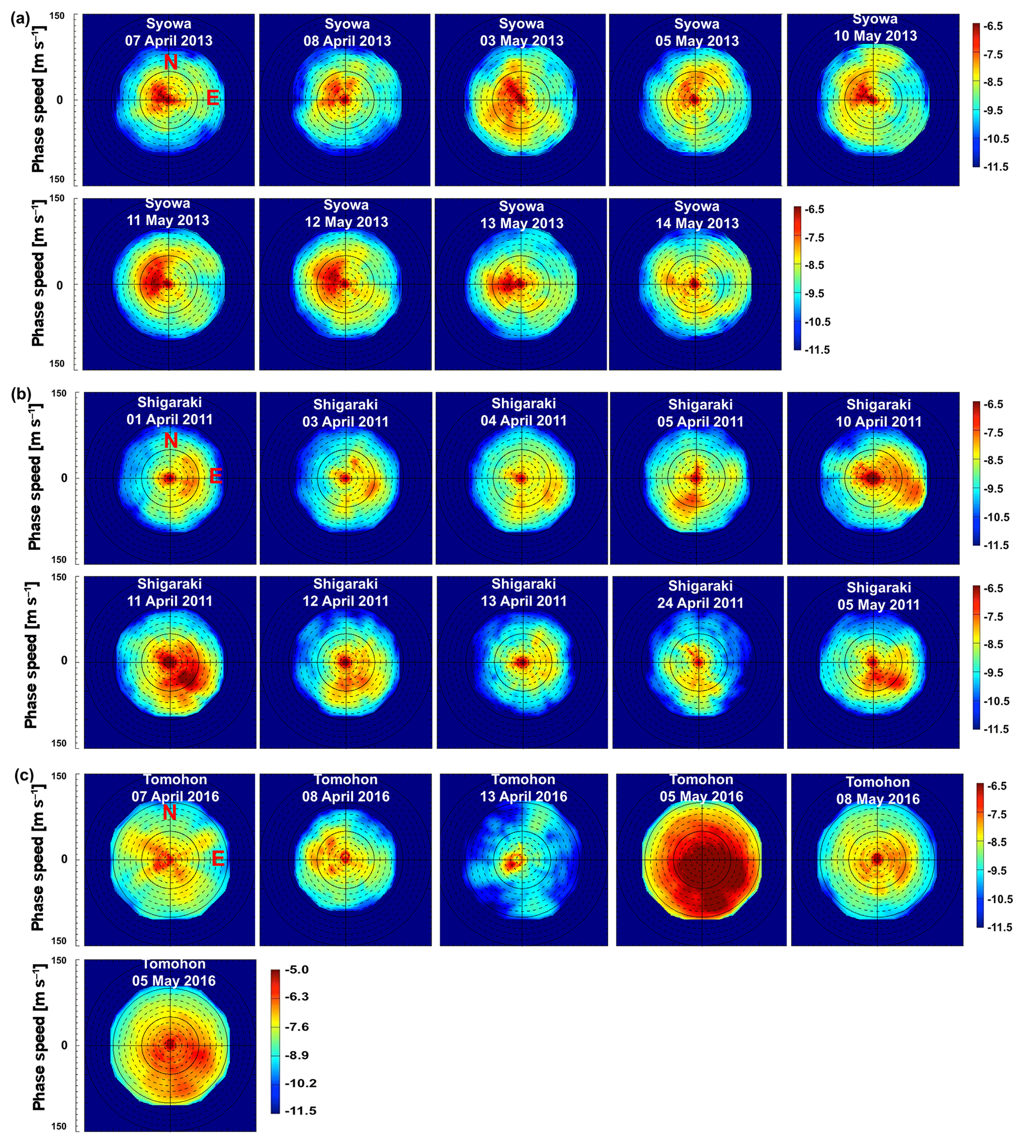
Figure 3Day-to-day variation of 2-D phase velocity spectra for April–May 2013 at the Syowa Station (a), in Shigaraki (2011) (b), and in Tomohon (2016) (c). Panel (c) is the same as that for 5 May 2016, but with a different color bar level to better visualize the dominant wave propagation direction.

Download

We observed 9 clear-sky nights at the Syowa Station from April to May 2013, 10 clear-sky nights in Shigaraki from April to May 2011, and 5 clear-sky nights in Tomohon from April to May 2016. The Syowa data were the same dataset as that reported by Matsuda et al. (2017). The image size for each observation site was 400×400 km and the sampling intervals (dt) were 1 min (Syowa), 5.5 min (Shigaraki), and 2.5 min (Tomohon). The different sampling intervals limit the maximum phase velocity to be analyzed; that at Shigaraki was the smallest. To avoid an aliasing effect on the 2-D phase velocity spectrum, we selected the period minimum (T_min) to be at least 2 times larger than the sampling interval (2×dt). In this study we set T_min to 3×dt. Because the dt of Shigaraki data was 5.5 min, we set the T_min to 16.5 min for all datasets to obtain the same frequency range. This setting can be easily altered by changing the input keyword (T_min) when running the function. The defaults were used for the other wave parameters.

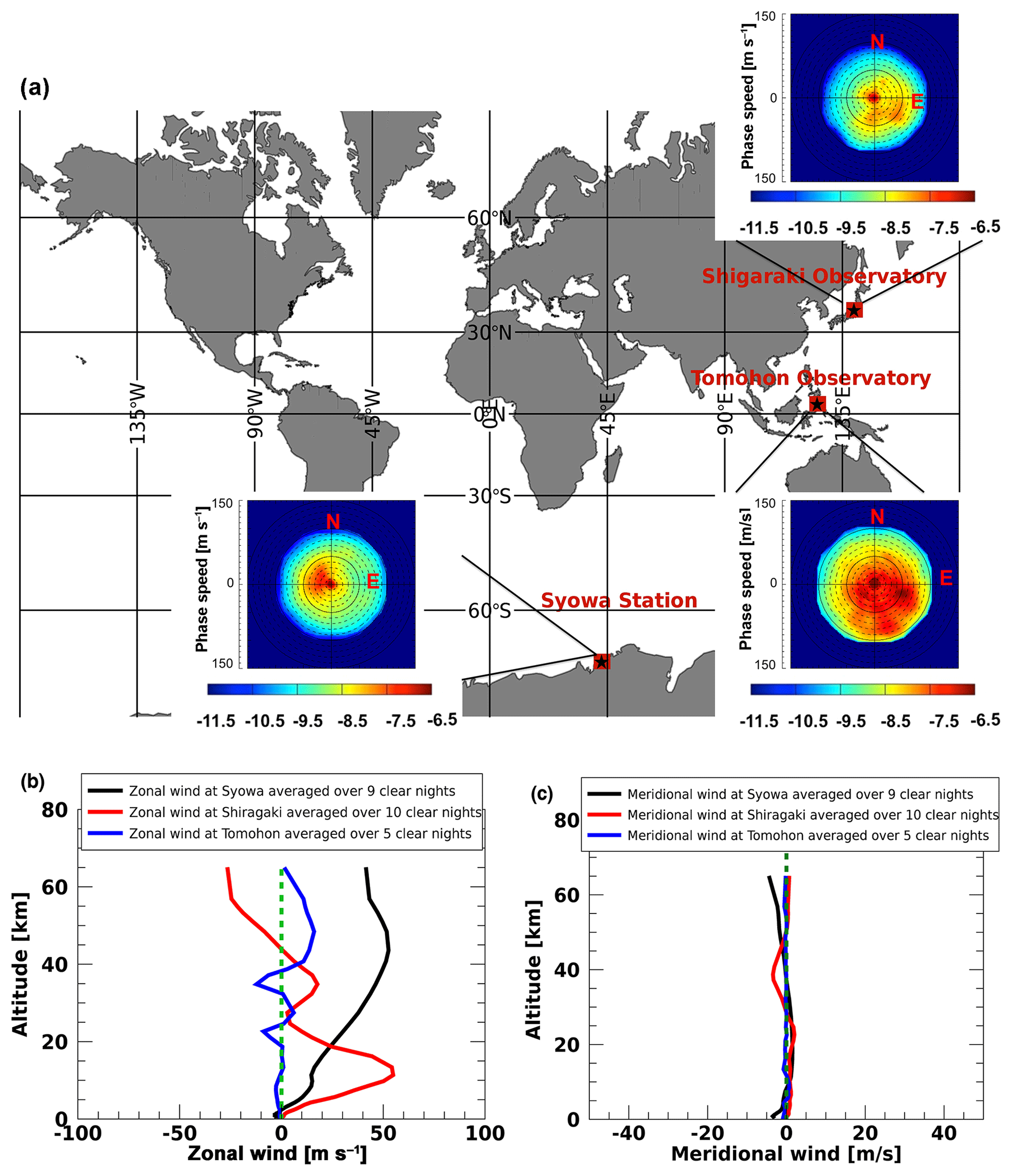
Figure 4(a) Average day-to-day variation of the 2-D phase velocity spectrum of AGWs observed at Syowa, in Shigaraki, and in Tomohon. (b) Average zonal wind profiles (positive: eastward) and (c) average meridional wind profiles (positive: northward) of GWs observed during clear nights from MERRA-2 data.

Download

Figure 3 shows the day-to-day variation of 2-D phase velocity spectrum results for (a) Syowa Station, (b) Shigaraki, and (c) Tomohon. The top and left represent the north and east respectively. The day-to-day plot at Syowa Station shows a lack of eastward gravity wave (GW) propagation and a dominant westward propagation, which is probably due to the filtering effect by the eastward polar night jet, as described in Matsuda et al. (2014). However, the azimuth direction with large power spectral density was not always the same; a much narrower azimuth distribution was observed on 13 and 14 May. This suggests that the distribution of the GW sources was limited on these days and changed from day to day. On the contrary, the 2-D phase velocity spectrum for Shigaraki shows a lack of westward propagation and dominant eastward and southward propagations. The strong spectrum based on Shigaraki data has a much larger day-to-day azimuth variation than that for Syowa, suggesting that the distribution of the wave source region varied more in Shigaraki, at least in this season's April and May. The day-to-day variation of the propagation direction was even stronger in Tomohon. At the same time, a significant day-to-day variation of the magnitude of the power spectrum was observed. The power was the weakest on 13 April; it was much stronger on 5 May and is overscaled in the plot. The last panel in Fig. 3c was plotted with the maximum color level; it is ∼30 times larger than the others. Such a significant day-to-day variation indicates the intermittency of the GWs.

Figure 4a shows the average nightly spectrum at each observation site plotted on the world map. The average phase velocity spectrum at the Syowa Station shows a distinct westward propagation with a phase speed below 50 m s⁻¹. In Shigaraki, AGWs propagate dominantly in the east-southeastward direction and reach phase speeds up to ∼80 m s⁻¹. The AGWs in Tomohon show a preferred propagation direction, that is, they are moving southeastward with phase speeds of up to ∼100 m s⁻¹. It should be noted that the plot for Tomohon is highly affected by a single day, 5 May. This also indicates the intermittency of GWs, which suggests that the net momentum transportation highly depends on the very strong GWs with smaller occurrence frequency.

One can discuss the AGW propagation by comparing the 2-D phase velocity spectrum and background conditions along the propagation path. Figure 4b and c show the zonal and meridional wind profiles, respectively, obtained from Modern-Era Retrospective Analysis for Research and Applications (MERRA-2; Gelaro et al., 2017) for each observation site. The profiles were averaged over the clear nights of the observed AGWs. The zonal wind over the Syowa Station, which was averaged over nine clear-sky nights, shows strong eastward wind up to ∼50 m s⁻¹ around ∼50 km, which could filter out the waves propagating eastward. A similar conclusion was reported by Matsuda et al. (2017), who applied a GW blocking diagram (Taylor et al., 1993; Tomikawa, 2015) by using horizontal wind data from MERRA and the medium-frequency (MF) radar to discuss the preferred wave propagation direction observed in the phase velocity spectrum. They concluded that eastward-propagating AGWs are restricted to propagating up to the mesopause due to critical-level filtering.

In contrast to the strong zonal wind at the Syowa Station, the average zonal wind profile in Shigaraki over 10 clear nights shows relatively weak westward wind with a speed of up to ∼30 m s⁻¹ at ∼50 km altitude. Previous studies of the seasonal directionality of AGWs in Shigaraki showed that east–west propagation anisotropy is usually caused by wind filtering of the mesospheric jet (e.g., Nakamura et al., 1999; Ejiri et al., 2003; Takeo et al., 2017). However, the westward wind in our current case for April–May 2011 is not stronger than 30 m s⁻¹ above the stratosphere; it is not strong enough to filter out all GWs with westward propagation. The average tropopause eastward jet is as strong as 60 m s⁻¹. If the GW source is associated with such an eastward jet structure, the horizontal phase velocity distribution of generated GWs should shift eastward. This could also be the reason for the lack of westward-propagating AGWs, especially those with higher phase velocities such as over 40 m s⁻¹.

The average zonal wind in Tomohon is small (<20 m s⁻¹) and likely has a limited impact on the much faster AGW phase speed (∼100 m s⁻¹). However, Fig. 4a shows that the GWs over Tomohon have a dominant southeastward propagation. As already discussed, this distribution is affected by the spectrum of a single day and should be highly affected by the location of the strong wave source on that day. Haffke et al. (2016) reported that the Intertropical Convergence Zone (ITCZ) is located above the Equator between March and April and starts to move north of the Equator in May, which could explain the dominant southward propagation of AGWs observed on 5 May 2016 (Fig. 3c). The scenario in which the distribution of the source location has a more significant effect on the AGW propagation direction than the background wind in the equatorial region agrees well with results reported by Nakamura et al. (2003). They reported AGW characteristics for Tanjungsari, Indonesia (107.9^∘ E, 6.9^∘ S) and based on the analysis of Geostationary Meteorological Satellite (GMS) data they concluded that the distribution of tropospheric clouds that are located mainly in the opposite direction of the wave propagation plays a more significant role than the relatively weak background wind. The meridional wind at each observation site has a weak velocity (<5 m s⁻¹) and likely has almost no impact on the wave propagation direction.

The M-transform function code and airglow data used in this study are stored in the NIPR repositories and can be provided on request. The MERRA-2 data used in the analysis can be freely accessed at https://disc.gsfc.nasa.gov/datasets/ (last access: 27 November 2018) (Gelaro et al., 2017).

The supplement related to this article is available online at: https://doi.org/10.5194/angeo-36-1597-2018-supplement.

SP developed the code, did the analysis and led the writing of the paper. TN came up with the original idea and contributed heavily to the discussion of the analysis results. MK did the preprocessing image of Syowa airglow data, helped modify the code and contributed to the discussion of the results. YT and MKE contributed to the discussion and helped edit the paper. KS provided the Shigaraki airglow data and contributed to the discussion of the results.

The authors declare that they have no conflict of interest.