the Creative Commons Attribution 4.0 License.
the Creative Commons Attribution 4.0 License.
 | 02 Oct 2018
Turbulent processes in the Earth's magnetotail: spectral and statistical research
Liudmyla V. Kozak
Bohdan A. Petrenko
Anthony T. Y. Lui
Elena A. Kronberg
Elena E. Grigorenko
Andrew S. Prokhorenkov
We use the magnetic field measurements from four spacecraft of the Cluster-II mission (three events from 2005 to 2015) for the analysis of turbulent processes in the Earth's magnetotail. For this study we conduct the spectral, wavelet and statistical analysis. In the framework of statistical examination, we determine the kurtosis for selected events and conduct extended self-similarity evaluation (analysis of distribution function moments of magnetic field fluctuations on different scales). We compare the high-order structure function of magnetic fluctuations during dipolarization with the isotropic Kolmogorov model and three-dimensional log-Poisson model with She–Leveque parameters. We obtain power-law scaling of the generalized diffusion coefficient (the power index that varies within the range of 0.2–0.7). The obtained results show the presence of super-diffusion processes. We find the significant difference of the spectral indices for the intervals before and during the dipolarization. Before dipolarization the spectral index lies in the range from to ( according to the Kolmogorov model). During dipolarization the type of turbulent motion changes: on large timescales the turbulent flow is close to the homogeneous models of Kolmogorov and Iroshnikov–Kraichnan (the spectral index lies in the range from −2.20 to −1.53), and at smaller timescales the spectral index is in the range from −2.89 to −2.35 (the Hall–MHD model). The kink frequency is less than or close to the average value of the proton gyrofrequency.
The wavelet analysis shows the presence of both direct and inverse cascade processes, which indicates the possibility of self-organization processes, as well as the presence of Pc pulsations.


The physical process responsible for the onset of magnetospheric substorms remains an unsolved mystery in spite of more than 5 decades of intense research efforts after the discovery of this episodic disturbance in the ionosphere and the magnetosphere. Many potential processes have been proposed by e.g. Nishida and Hones (1974), Rostoker and Eastman (1987), Samson (1998), Rothwell et al. (1988), Lui et al. (1991), Haerendel (1992), Kan (1998), and Streltsov et al. (2010). Soon after the turn of the century, two prominent scenarios of substorm development emerged with different emphasis on the initial substorm onset location and the associated physical mechanism (Baker et al., 1996). The first model is the Near-Earth Neutral Line (NENL) model with the onset location in the middle of the tail at distances of 15–30 Earth radii in which a large-scale process involving reconnection of magnetic field lines is invoked by Baker et al. (1996) and Nishida (1978). The second one is the Current Disruption (CD) model in which a plasma instability at distances of 6–15 Earth radii is invoked initially by Lui (1991), Roux et al. (1991), and Samson (1998), followed by magnetic reconnection at further downtail distances (Lui, 1991). The distinguishing characteristics of these two scenarios are the initial onset location and the associated physical process.
A four-satellite ESA mission, named Cluster-II, and a five-satellite NASA mission, named Time History of Events and Macroscale Interactions during Substorms (THEMIS), were launched to identify the location where the substorm disturbances are initiated in the magnetotail (Angelopoulos, 2008).
The strategy adopted by these missions is to have some satellites situated at different downtail distances to identify the originating location of substorm disturbance. This strategy turns out not to be foolproof as magnetic reconnection was later recognized to be localized in the local time extent and not a large-scale process as originally envisioned (Nakamura et al., 2004). Because of the spatial limitation of magnetic reconnection, satellite observations have not led to a compelling conclusion to settle the mystery as observations of the propagation direction of substorm disturbances in the tail yielded diversified results with many reports on results to be consistent with one or the other of the scenarios, i.e. no consistency with one particular model (Akasofu, 2012, 2017; Angelopoulos, 2008; Hwang et al., 2014; Lui, 2009; Panov et al., 2013). A complication in distinguishing the two scenarios is the presence of the so-called pseudo-breakups (Lopez, 1990; Lui, 2002, 2004; Runov et al., 2012; Zelenyi and Veselovskiy, 2008).
On the other hand, both scenarios have common consequences such as impulsive particle acceleration, dipolarization, and formation of a current wedge (Lui, 2004; Zelenyi and Veselovskiy, 2008). Several plasma instabilities have been proposed to play a role in these substorm scenarios. External and internal plasma environments with the presence of heavy ions affect the occurrence of these instabilities. Instabilities in the CD model include the ballooning instability (Cheng and Lui, 1998; Roux et al., 1991) and the cross-field current instability (Lui, 2004). Although magnetic reconnection is not a plasma instability process, it requires an instability such as ion tearing instability (Schindler, 1974; Sitnov and Schindler, 2010) to form an X-line for its existence. Besides, magnetic reconnection can involve turbulence, but one should not forget about the work of Speiser (1970) describing the magnetic reconnection without noise (i.e. turbulence). Heavy ions play a significant role in the development of substorms since their presence changes current sheet thickness and its structure, leading to favourable conditions for magnetic reconnection and the generation of Kelvin–Helmholtz instability (Kronberg et al., 2014, 2017a, b).
Investigation of the magnetotail is significantly complicated by the presence of turbulence due to instability resulting in a “catastrophic” alteration of the flow and magnetic field structure (Barenblatt, 2004; Frik, 1999; Frisch, 1995). Complex turbulent processes that occur in the Earth's magnetosphere cannot be described within the analytical MHD flow models. To consider the properties of turbulence at different temporal and spatial scales, one should adopt methods of statistical physics and the cascade model developed in hydrodynamic theories. Also note that, when considering a statistical system to be characterized by self-similarity, it can be regarded as a physical characteristic of a fractal size equal to the effective Larmor radius of particles and properties of turbulent processes associated not only with the physical mechanisms of instability, but also with symmetries that describe the scale invariance (Chen et al., 2017; Savin et al., 2011).
An analytical or numerical solution of the turbulent plasma dynamics (in three-dimensional geometry) and determination of turbulence features at large timescales are not currently possible. Therefore, statistical properties of turbulence associated with large-scale invariance are determined experimentally along with estimation of spectral indices in the assumption of power laws for plasma parameters. This allows one to get an idea of the physical properties of plasma turbulence and a description of the transport processes in the turbulent regions in qualitative and quantitative terms (Hadid et al., 2015; Kozak et al., 2012, 2015). This approach has yielded important insights into the turbulent plasma characteristics, mainly in the magnetosheath. Plasma turbulence in the magnetotail is a key feature for dipolarization in the CD model. The multiscale nature of plasma turbulence at a CD site has also been explored by analysis from the non-linear dynamics approach or from wave identification by e.g. Lui and Najmi (1997), Consolini and Lui (1999, 2000), Lui (2002), Consolini (2005), Lui et al. (2008), Yoon et al. (2009), Le Contel et al. (2009), Zhou et al. (2009), and Mok et al. (2010).
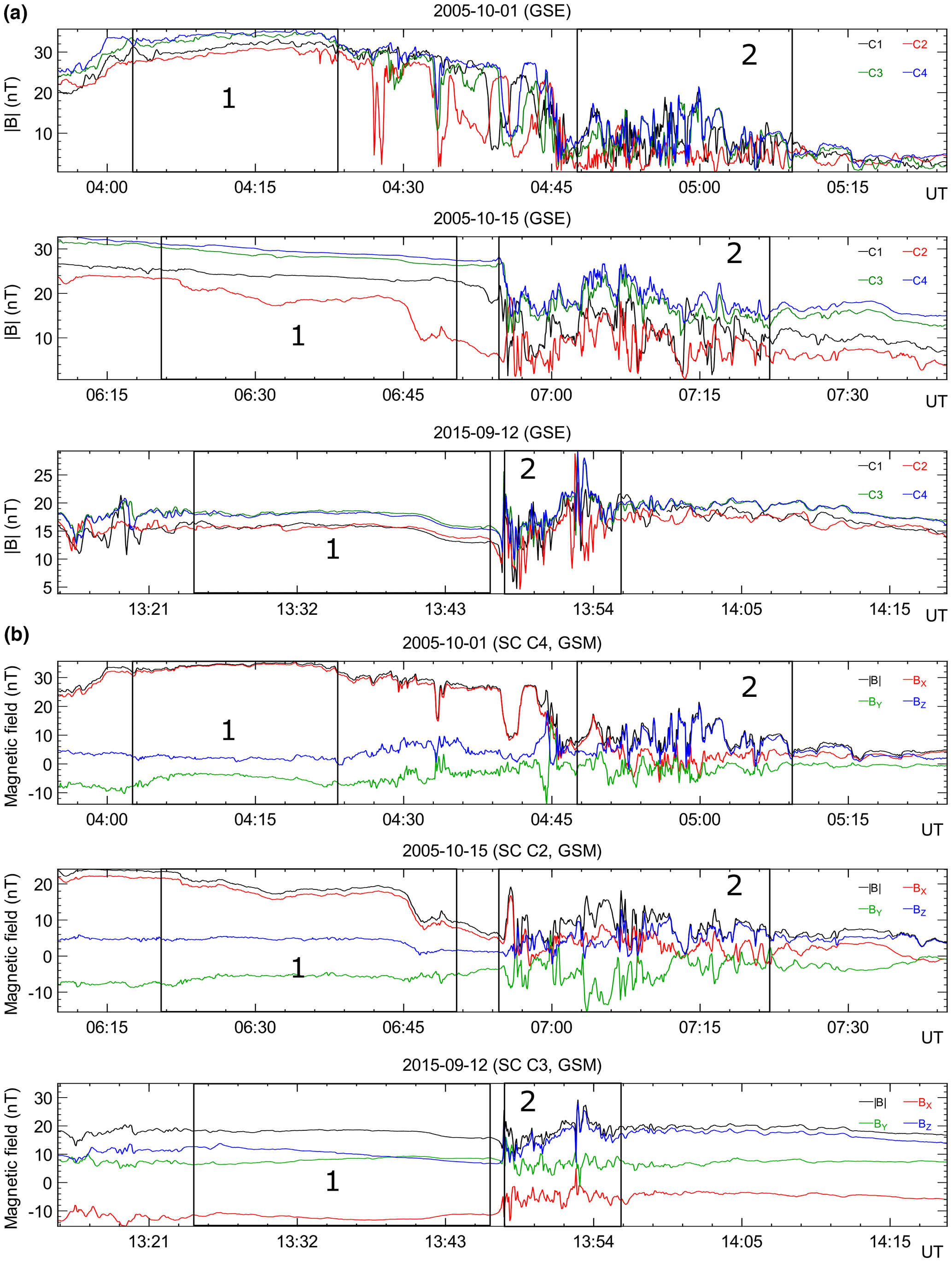
Figure 1(a) Absolute values of the magnetic field in GSE. 1 – intervals for the moments before dipolarization; 2 – intervals during the dipolarization of the magnetic field. (b) Examples of magnetic field dipolarizations in GSM. The observations are shown from satellites closest to the current layer. 1 – intervals for the moments before dipolarization; 2 – intervals during the dipolarization of the magnetic field.
In this work, the spectral and statistical approach was carried out to examine the features of the magnetic field dipolarization in the Earth's magnetotail for three events (12 September 2015, 15 October 2005, 1 October 2005). The methods and approaches used in the work are described in detail and tested in the works by Kozak and Lui (2008), Kozak et al. (2011, 2012, 2015, 2017), Savin et al. (2011, 2014), and Kronberg et al. (2017a). Acceleration processes of protons and electrons associated with wave activity observed during dipolarization events in 2005 were previously studied in papers by Grigorenko et al. (2016). This work provides the statistical review estimates on the features of turbulent and dynamic processes at small timescales.
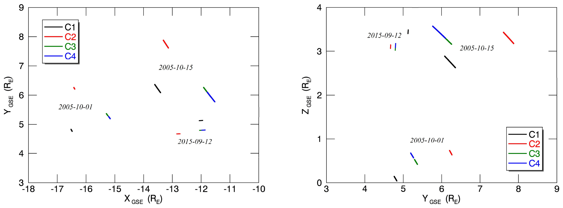
The data of the magnetic field for this analysis were obtained by the spacecraft (SC) of the Cluster-II mission in the near-Earth tail for three events (two events in 2005 and one event in 2015) during the dipolarization of the magnetic field (see Fig. 1a, b). The sampling rate is 22.5 Hz. The magnetic field data are obtained by the fluxgate magnetometer (FGM) (Balogh et al., 2001). In the course of the study, the peculiarities were considered of the magnetic field fluctuations for moments prior to dipolarization (relative level of fluctuations ∼0.05–0.24 (interval 1) and during the dipolarization of the magnetic field (relative fluctuation level ∼0.8–1 (interval 2) (Fig. 1a, b). The spacecrafts were at the geocentric distances 11–17 RE in the anti-sunward direction in the pre-midnight sector (Fig. 2).
The event of 2015 satisfies the most the conditions of dipolarization for the CD model by Lui (2018). For the CD model, large magnetic fluctuations predominantly occur around the neutral sheet of the magnetotail where . During CD, the level of magnetic fluctuations can reach the order of one or more, where is the Bz value before CD onset. This type of event typically lasts for several minutes. The Bz component could become negative, in spite of a strong background positive Bz component from the dipole magnetic field. It is accompanied by particle energization and intense fluctuating electric fields. The cross-tail current breaks up into filaments and may reverse its direction. The associated plasma flow pattern is not organized by the Bz polarity, unlike magnetic reconnection.
In the dipolarization region the fluctuations of the magnetic field greatly differ from the region before dipolarization: in particular for the event on 1 October 2005 the magnetic field variations normalized to the current mean value are –1, , , and –1; for the event on 15 October 2005 – –0.5, –1, –0.8, and –1; for the event on 12 September 2015 – –1, –0.7, –1, and –1.
Fu et al. (2012)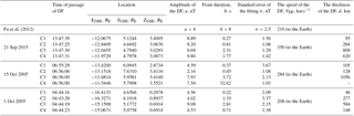
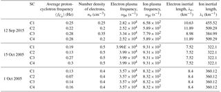
Table 2Estimated values of plasma characteristics in the dipolarization region.
Since the region of dipolarization is traced by four space vehicles, we were able to estimate the speed and direction of the dipolarization front (DF) motion, the thickness of the front (Table 1). The estimated values of plasma characteristics in the dipolarization region (interval 2) are collected in Table 2.
Moreover, according to Fu et al. (2012), during the dipolarization the variation of Bz for different satellites can be represented as
where represents the interval from 60 s before to 15 s after the dipolarization front. a, b, and c are fitting coefficients, and σ is a standard error.
The calculated values of the coefficients are also given in Table 1.
3.1 Spectral analysis
Within the spectral analysis, the spectral power density (PSD) was built from the frequency f, and the power-law dependence PSD(f)∼fa was determined. To determine the PSD of the signal for a series of N measurements Xn, a discrete Fourier transform (Daly and Paschmann, 2000) was used:
where , .
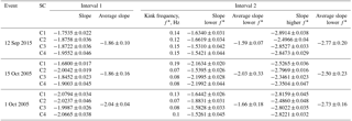
To find the break points and the slope of the spectrum, we used a piecewise linear approximation of logPSD from log(f) in the frequency range 0.005–∼1.0 Hz for the pre-dipolarization interval and 0.01–3.0 (events 1 October 2005 and 15 October 2005) and 0.01–1.0 (event 12 September 2015) Hz for dipolarization. The limitation of frequencies at a high level is due to the presence of instrumental noise, and at the low-frequency range due to the amount of data sampling and the edge effect of the smoothing procedure. The PSD results for the absolute value of the magnetic field are shown in Fig. 3 and Table 3.
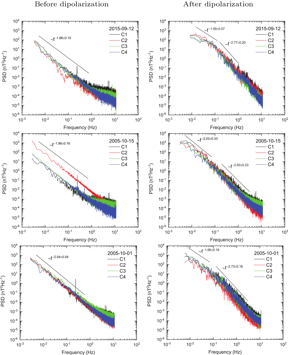
During the time before the dipolarization (interval 1), for all events and spacecrafts, there is no sharp change in the PSD power law in the inertial interval (the exponent varies in the range from −2.08 to −1.68). During dipolarization (interval 2), the situation is significantly different. There is an increase in the “steepness” of PSDs for higher frequencies than the kink frequency, which means more efficient energy transfer from large to smaller scales. For practically all spectra of interval 2, the kink frequency is less than or close to the average value of the proton gyrofrequency (Table 2). The kink frequency determines the characteristic frequency of the type change (i.e. the energy transfer rate) of the turbulent cascade in the inertial range. In particular, for events 12 September 2015 and 15 October 2005 the break corresponds to about half of the proton frequency ωc∕2. The fact that the break is observed at frequencies smaller than the proton gyrofrequency may indicate a significant effect of heavy ions at the distances considered (according to the measurements of the density by the CIS instrument (Rème et al., 2001) for event 1 October 2005, in the region of the magnetic field dipolarization, the percentage of oxygen ions in relation to protons () is 21.1±10.0 % (SC C3) and 9.3±1.5 % (SC C4), and the percentage of helium in relation to protons () (SC C3) and (SC C4); for event 15 October 2005 – (SC C4) and (SC C4); for the 12 September 2015 event – (SC C4) and (SC C4)). At the same time, the exponent lies in the range from −2.2 to −1.53 on large timescales of , and at smaller timescales ωc∕2–3 Hz, the value lies in the range from −2.89 to −2.35. The greatest difference at different timescales is observed for the 2015 event.
3.2 Wavelet analysis
Within the framework of the wavelet analysis for a series of measurements Xn () with time step δt, a Morlet wavelet (Torrence and Compo, 1998) was used:
where ω0 is the dimensionless frequency, and η the dimensionless time.
The continuous wavelet transform of the discrete signal Xn is defined as the convolution of the mother wavelet whose argument is scaled and transmitted with a signal (Farge, 1992; Grinsted et al., 2004; Jevrejeva et al., 2003):
where (*) is the complex conjugate, is the wavelet power spectrum, and s is the wavelet scale. Index 0 in Ψ0 denotes that the function is normalized.
The results of the continuous wavelet transform of the magnetic field module in the dipolarization region are shown in Figs. 4 to 6. The time range was chosen to include the dipolarization interval (interval 2) with some margin (±5 min) to exclude the influence of the edge effects of the wavelet transform on the explored intervals. The upper limit of the wavelet transform is limited by the Nyquist frequency. The sampling frequency of the measurements makes it possible to analyse the presence of high-frequency fluctuations in addition to the low-frequency components.
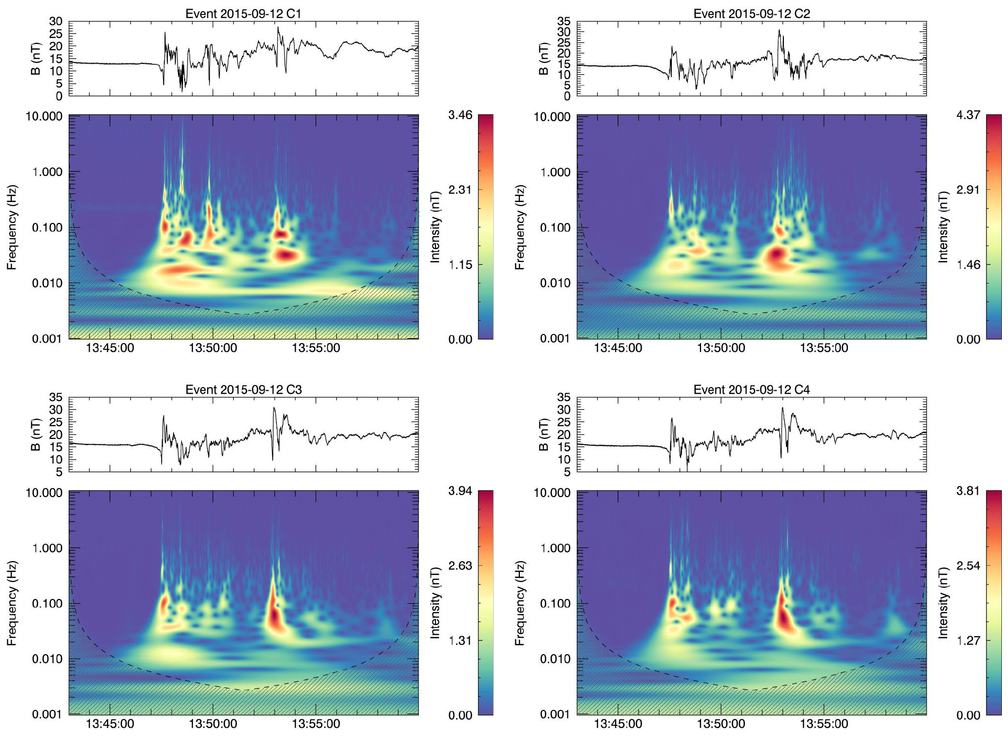
Figure 4The results of wavelet analysis for event 12 September 2015. The cone of influence is shown by the shaded region.

Figure 5The results of wavelet analysis for event 15 October 2005. The cone of influence is shown by the shaded region.
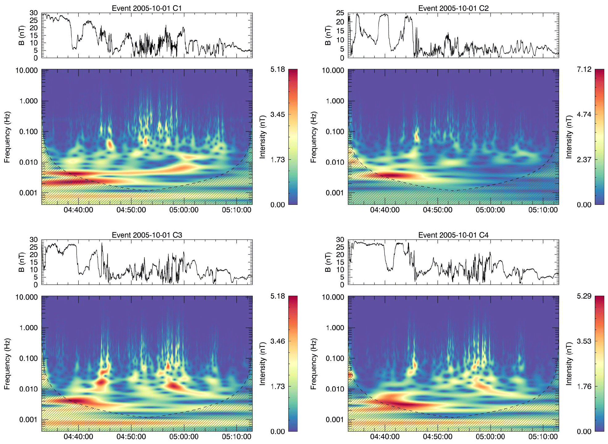
Figure 6The results of wavelet analysis for event 1 October 2005. The cone of influence is shown by the shaded region.
In Fig. 4 the wavelet analysis of the magnetic field magnitude for the event on 12 September 2015 is presented. In this case C3 and C4 were located ahead of C1 and C2, with C2 being the furthest in the magnetotail. Inverse and direct cascades are present in wavelet analysis at multiple times: 13:47:30 (dipolarization onset) and 13:53:00, both spanning 0.02–0.2 Hz in the frequency domain. This signal broadens for C1 and C2 wavelets and breaks up into smaller time-frequency forms: e.g. the signal on 13:53:00 UT becomes stronger in time and frequency domains of 1 min and 0.01 Hz correspondingly. Wavelet transform for C1 is characterized by a prevalence of intensity enhancements in the wide frequency range at an earlier stage of the turbulent phase of dipolarization at 13:47:30–13:50:30 as compared to transforms for C2, C3, and C4. Also for C1, it is interesting to note the fact of coexistence of the inverse and direct cascades simultaneously starting at 13:47:30, and wherein the first one lasts for 2 min with frequency decrease from 0.015 to 0.008 Hz and the more intense second one lasts for 2.5 min with slight frequency increase from 0.015 to 0.02 Hz.
Figure 5 presents the wavelet transform for event 15 October 2005. Taking into account the cone of influence (COI), there are no strong enhancements presented for C3 and C4. For both these satellites, only high-frequency short signals are present. Transformations for C1 and C2 have a much richer frequency content. The component 0.008–0.01 Hz is present on all wavelet analysis, with the maximum amplitude shown at the C2 satellite. For C1 this signal has a broader structure, starting from 06:56 until 07:18, with frequency spanning from 0.005 to 0.02 Hz. Both of the satellites hold the same structure of short-term high-frequency signals up to 1 Hz.
Figure 6 demonstrates the wavelet analysis for the event on 1 October 2005. The third and fourth SCs were located relatively close, with the first and second slightly behind in the magnetotail. Although the onset of dipolarization begins at 04:49, where the Bz component becomes comparable with magnetic field magnitude B, the signal up to this moment is not devoid of high-amplitude changes. Transforms for C3 and C4 show strong signals in the frequencies ranging from 0.002 to 0.004 Hz, which span 10 min, with different times for intensity maxima: 04:39 for the third SC and 04:42 for the fourth. In both cases, a structure of inverse cascade can be traced before dipolarization onset: the frequency decreases from 0.005 to 0.002 Hz. The second inverse cascade lasts for 10 min starting from 04:57 in the time domain with a gradual decrease in the frequency range from 0.015 to 0.005 Hz, while at higher frequency it breaks up into smaller wave forms. Wavelet decomposition for C2 differs from the others, primarily by the absence of any cascade during the turbulent phase of dipolarization with a distinct component at 0.0035 Hz which spans for 8 min. It is interesting to note that just for this SC the spectral slope of the PSD spectrum is less in absolute value in comparison with other SCs: −2.5 against −2.8. The relatively short components, with durations of less than 2 min, extend in the frequency range from 0.02 up to 0.2 Hz. For C1 there is an enhancement with long duration at 0.004 Hz, which spans more than 20 min, and one with a gradual increase in frequency up to 0.007 Hz, i.e. direct cascade. Such prolonged intensity enhancements are observed with a wide frequency coverage beginning with 0.002 up to 0.01 Hz. A large number of high-frequency components appears in measurement signals from both satellites.
Thus, during the dipolarization, the magnetometers of all spacecraft recorded powerful signals with periods of 50, 100, 125, 166, and 200 s, corresponding to Pc4 (45–150 s) and Pc5 (150–600 s) pulsations, as well as direct and inverse cascade processes. The presence of inverse cascade processes indicates that together with the decay of the vortex structures, self-organization also takes place, i.e. smaller vortices are grouped into larger vortices. In the analysed events Pc pulsations were observed by all satellites – in the spatial range of 11–17 RE. The largest number of cascade processes is observed at a distance of 15–16 RE, and the largest number of inverse cascades is in the range 13–14 RE.
3.3 Statistical analysis
In the presence of intermittency in magnetic field fluctuations, the energy cascade is characterized by non-homogeneous non-linear transfer of energy among smaller and smaller structures, with the result of concentrating the energy on limited regions of space.
This effect becomes more and more intense at smaller and smaller scales. More properly, intermittency corresponds to scale-dependent, non-Gaussian, heavy-tailed probability distribution functions (PDFs) of the field fluctuations (Frisch, 1995). Non-Gaussianity of the PDFs, which increases as the spatial scale decreases, is indeed due to the presence of the intense, phase-correlated fluctuations, due to the transfer of energy between contiguous eddies. It should be pointed out that spectral properties of the field are not essentially affected by intermittency. This is normally studied through the scaling properties of PDFs, or through their high-order moments (the structure functions), for which models and theoretical results exist (Frisch, 1995). The observation of intermittency implies that a non-linear, non-homogeneous energy transfer takes place in the system (Zimbardo et al., 2010).
In order to determine the presence of intermittence, an analysis of the value of the excess for all the SCs of the considered events has been performed, and the Hölder parameter h for spacecraft C1 has been determined. In this case, the statistical properties of the magnitude value of the magnetic field fluctuations at different timescales were analysed. The use of the Taylor hypothesis for various regions of the magnetospheric tail is detailed in Borovsky and Funsten (2003).
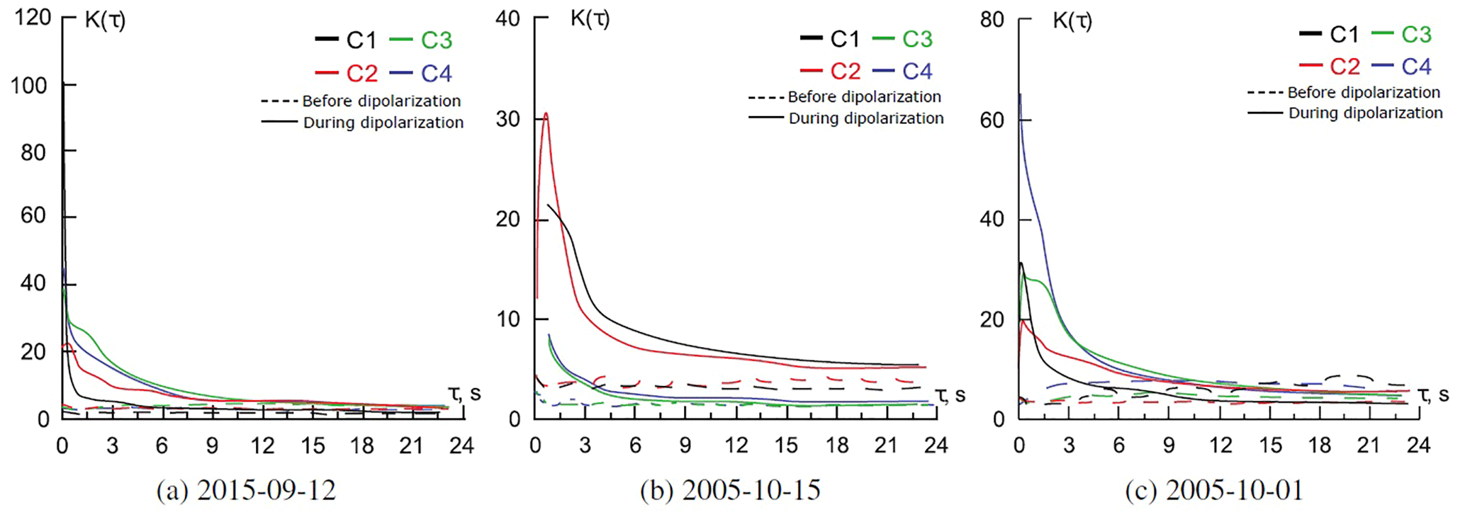
The value of the kurtosis was determined by the moments of the second and fourth orders from the formula by Zacks (1971):
where is the structure function of qth order, 〈…〉 is the time average of the data, τ is the timescale (time shift), multiple of measurements discretization 0.0445 s. When determining the excess value of the magnetic field fluctuations, the dependence of the functions K(τ) from the scale parameter τ was constructed. The significance of excesses for different mission SC and different events is shown in Fig. 7. It is clearly seen from the graphs that for the interval 1 (dotted line) for almost all satellites the value of K(τ) varies about 3 (in the range from 2 to 5), which is close to the normal distribution. The only exception is the measurement on the C1 spacecraft for 1 October 2005. Also, for interval 1, the spin tone of SC rotation is clearly observed by sheer accident near the gyrofrequency. For the dipolarization region (interval 2, solid line), the function K(τ) on small scales varies from 100 (C1, 12 September 2015) to 8 (C3, C4, 15 October 2005).
For SC C3 and C4, changes in the value of kurtosis are very similar. The largest jump is observed for C1, 12 September 2015. A sharp drop in the kurtosis is observed on the scales to the ion-cyclotron frequency (Table 2).
The “gap” of values for interval 2 for very small τ can be explained by the instrumental error of observations.
Thus, for a region of dipolarization at small timescales, we have a distribution with a sharper vertex and broad wings (the excess value is greater than 3) than for a normal distribution.
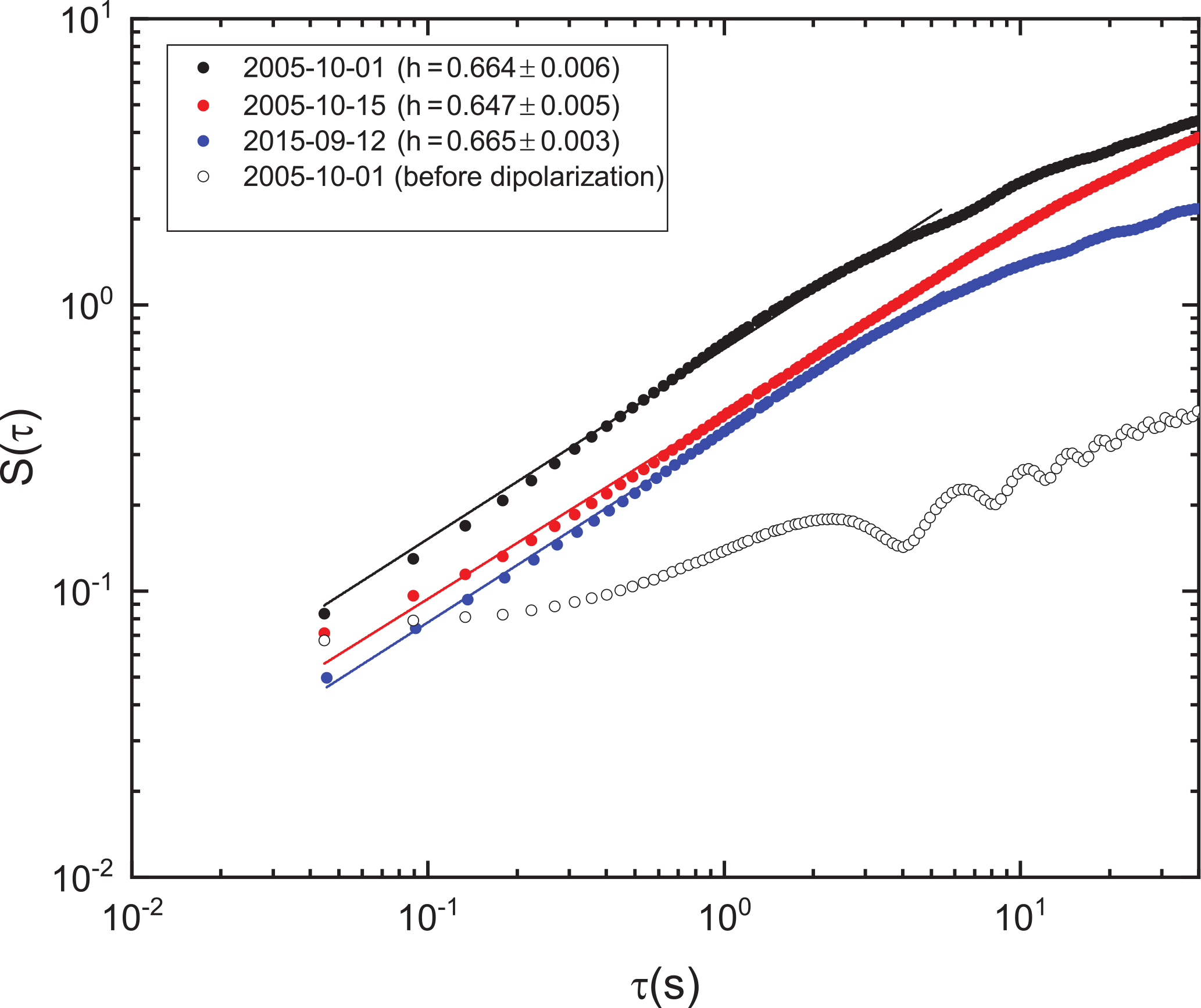
The presence of intermittency is indicated by the analysis of the first-order structure function (Fig. 8). For a self-affine signal, , where h is the Hölder exponent (note that the Hölder exponent is the Hurst exponent of first order, h=0.5 for Brownian motion). The higher value of h afterward indicates a persistent signal with a longer correlation than a random noise and may imply the occurrence of reorganization during dipolarization (Chang, 1992; Consolini and Lui, 2000). In our case, the Hölder exponent is in the range at the time of dipolarization.
Also, for the interval prior to dipolarization, the variations “caused” by the presence of spacecraft spin effects in the data are clearly visible.
To compare the type of turbulent processes with the available models of turbulent processes, an analysis of the high-order structural function was done, allowing one to characterize the properties of heterogeneity at small timescales.
In this case, the structural function is determined by the ratio:
where 〈…〉 is the time average of the data, and τ is the time step.
The existence of the criterion of generalized self-similarity for an arbitrary pair of structural functions allows one to find ζ(q) and estimate the types of turbulent and diffusion processes (Dubrulle, 1994). In this case, the non-linear functional dependence ζ(q) from the order of the moment q for experimental data is a consequence of the intermittency of processes. For the interpretation of the non-linear spectrum ζ(q), the log-Poisson model of turbulence is used, in which the power index of the structural function is determined by the relation (Dubrulle, 1994; Kozak et al., 2011; She and Leveque, 1994)
where β and Δ are parameters that characterize intermittency and singularity of dissipative processes, respectively. It is important to note that within the framework of this model a stochastic multiplicative cascade is considered, and the logarithm of dissipation energy is described by the Poisson distribution. For isotropic three-dimensional turbulence, (SL) (She and Leveque, 1994).
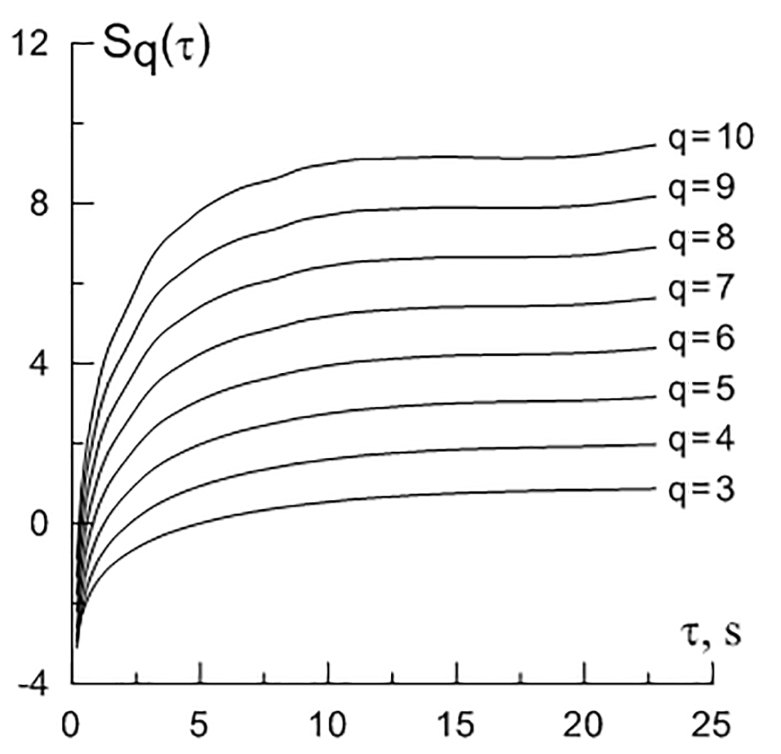
Figure 9Dependence of the order of the structure function for different timescales during dipolarization (event 15 October 2005).
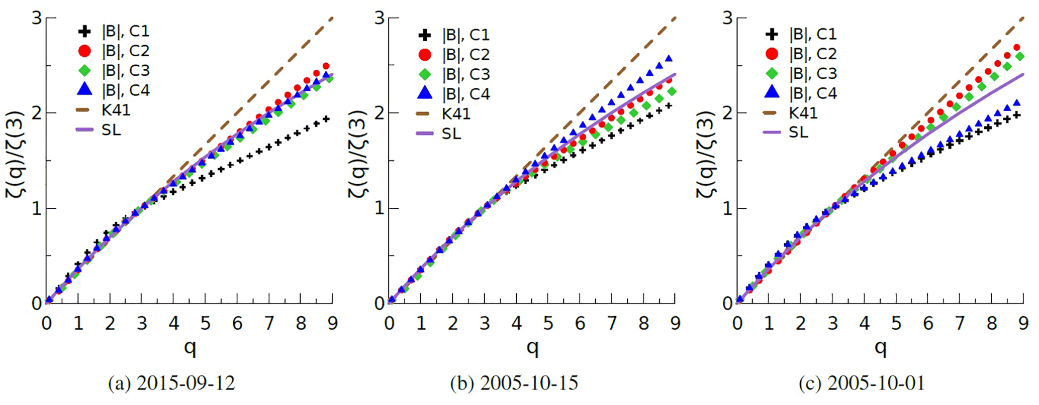
Figure 10The results of ESS analysis (during DP). Ratio of the power of the qth-order structural function to the third-order function power. The experimental data for the magnetic field are marked with the symbol; the solid line corresponds to the value calculated using the formula in the log-Poisson cascade model for (SL), and the dotted line corresponds to the q=3 (K41).
The power law of the type Sq(τ)∼τζ(q) (i.e. self-similarity – linear dependence) is observed on limited timescale intervals (Fig. 9). For the considered satellite measurements, this interval is close to the value of the ion-cyclotron frequency during dipolarization (Table 2).
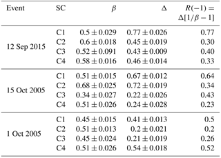
The results of scaling the moments of the probability density function for different orders of q in the analysis of small-scale turbulence and comparing them with the Kolmogorov model are shown in Fig. 10. The results of the ESS analysis of the satellite measurements indicate the heterogeneity of turbulent processes during the dipolarization to describe what can be a log-Poisson cascade model with fitting parameters. The obtained values of the parameters β and Δ are given in Table 4. In addition, the obtained values can be used to determine the characteristics of the diffusion transfer of plasma. In this case, the properties of diffusion are considered within the concept of a multi-fractal multiplicative cascade (Lovejoy et al., 1998). The coefficient of generalized diffusion is determined by the parameters of the structural function ζ(q) (intermittency and singularity) by the relations by Lovejoy et al. (1998) and Prokhorenkov et al. (2015):
This approach is used to estimate the transfer in a statistically inhomogeneous medium, and the index R, in general, is determined by the fractal properties of the medium and characterizes (on average) the topological properties (connection properties that determine the transfer) of a stochastic structure of turbulence.
The resulting values of R lie within the range from 0.20 to 0.77 (Table 4). Given that the law of particle displacement over time is given by the formula by Treumann et al. (1990), Chechkin et al. (2008), and Zaburdaev et al. (2015), with an indicator –1.77>1, this dependence means the existence of super-diffusion.
As a result of the analysis, it can be concluded that the relative variations of the magnetic field during the dipolarization exceed the value before dipolarization by more than 5 times. The distribution functions of magnetic field fluctuations during the disruption of the current layer indicate the non-Gaussian statistics of processes, as well as the excess of large-scale perturbations generated by the source.
Comparing the structure functions of the magnetic field fluctuations during dipolarization with the Kolmogorov model, it is impossible to describe turbulent processes on small timescales using a homogeneous model. Using the coefficients of intermittency and singularity of turbulent processes found in the ESS analysis, the power law of the generalized diffusion coefficient on the scale was obtained (the power index varies within the range from 0.2 to 0.77), indicating the presence of super-diffusion processes.
One of the important results is the significant difference of the spectral indices for the intervals before and during the dipolarization. Before dipolarization the spectral index lies in the range from to ( according to the Kolmogorov model), and during dipolarization the type of turbulent motion changes: on large timescales the turbulent flow is close to the homogeneous models of Kolmogorov (1941) and Iroshnikov–Kraichnan (1959) (the spectral index lies in the range from −2.20 to −1.53), and at smaller timescales the spectral index lies in the range from −2.89 to −2.35 (the Hall–MHD model). The kink frequency is less than or close to the average value of the proton gyrofrequency. The Hall–MHD model includes the Hall term in the magnetic induction equation. The Hall term is proportional to the ion inertial length c∕ωpi, which means this term is important for the small scales (Galtier and Buchlin, 2007). Both the standard MHD and the electron MHD can be recovered from Hall–MHD by taking appropriate limits. By considering magnetic turbulence spectra for scales smaller than c∕ωpi, Galtier and Buchlin (2007) found a number of spectral indexes, which go from when magnetic energy dominates kinetic energy to when kinetic energy dominates magnetic energy.
Also, within the framework of the research the following results were obtained:
-
the higher the PSD value, the greater the value of the height of the excess;
-
the log-Poisson model of turbulent processes with She–Leveque parameters corresponds to variations in the value of K(τ) in the range of 30–40; and
-
the spectral indices correlate with the values of the diffusion coefficient.
The wavelet analysis showed the presence of both direct and inverse cascade processes, as well as the presence of Pc pulsations. The presence of Pc pulsations in the region of dipolarization was also discussed in Panov et al. (2013, 2015).
Thus, during dipolarization the large-scale and multi-fractal disturbances of the magnetic field are observed and the presence of inverse cascade processes also indicates the possibility of self-organization processes.
In this paper we only used open-access data. The Cluster data were downloaded from the Cluster Science Archive version 2.0 at https://csa.esac.esa.int/csa-web/, last access: 20 August 2018. To obtain the data, one should start the CSA GRAPHICAL USER INTERFACE, and then to download the data, the particular instrument and time interval should be selected.
LVK formulated the goal and tasks of the investigations, carried out the statistical and spectral analysis of features of the magnetic field fluctuations in the Earth's magnetosphere tail, and also carried out the analysis of obtained results and calculated characteristics of the turbulent processes. BAP selected the considered work events and conducted the spectral and wavelet analysis of the data of the Cluster-II mission. ATYL carried out analysis of the obtained results. EAK and EEG selected and analyzed the dipolarization events used for the subsequent analysis of turbulence properties. ASP took part in the wavelet analysis of the data. All authors took part in the discussion about obtained results and preparation the article for publication.
The authors declare that they have no conflict of interest.
The work was conducted in the framework of a complex programme of the National Academy of Science of Ukraine in Plasma Physics, with support of the the education programme of Ministry of Education and Science of Ukraine no. 2201250 “Education, Training of students, PhD students, scientific and pedagogical staff abroad”, grant Az. 90 312 from the Volkswagen Foundation (“VW-Stiftung”) and the International Institution of Space Research (ISSI-BJ).
We also thank the Principal Investigators and teams of FGM and CIS instruments of the Cluster mission.
Edited by:
Elias Roussos
Reviewed by: Gaetano Zimbardo and one anonymous
referee
Akasofu, S.-I.: Auroral Morphology: A Historical Account and Major Auroral Features During Auroral Substorms, in: Auroral Phenomenology and Magnetospheric Processes: Earth and Other Planets, 29–38, American Geophysical Union, Washington, D.C., USA, https://doi.org/10.1029/2011gm001156, 2012. a
Akasofu, S.-I.: Where is the magnetic energy for the expansion phase of auroral substorms accumulated? 2. The main body, not the magnetotail, J. Geophys. Res.-Space Phys., 122, 8479–8487, https://doi.org/10.1002/2016ja023074, 2017. a
Angelopoulos, V.: The THEMIS Mission, Space Sci. Rev., 141, 5–34, https://doi.org/10.1007/s11214-008-9336-1, 2008. a, b
Baker, D. N., Pulkkinen, T. I., Angelopoulos, V., Baumjohann, W., and McPherron, R. L.: Neutral line model of substorms: Past results and present view, J. Geophys. Res.-Space Phys., 101, 12975–13010, https://doi.org/10.1029/95ja03753, 1996. a, b
Balogh, A., Carr, C. M., Acuña, M. H., Dunlop, M. W., Beek, T. J., Brown, P., Fornacon, K.-H., Georgescu, E., Glassmeier, K.-H., Harris, J., Musmann, G., Oddy, T., and Schwingenschuh, K.: The Cluster Magnetic Field Investigation: overview of in-flight performance and initial results, Ann. Geophys., 19, 1207–1217, https://doi.org/10.5194/angeo-19-1207-2001, 2001. a
Barenblatt, G. I.: Turbulent boundary layers at very large Reynolds numbers, Russ. Math. Surv.+, 59, 45–62, 2004. a
Borovsky, J. E. and Funsten, H. O.: MHD turbulence in the Earth's plasma sheet: Dynamics, dissipation, and driving, J. Geophys. Res.-Space Phys., 108, https://doi.org/10.1029/2002JA009625, 2003.
Chang, T.: Low-dimensional behavior and symmetry breaking of stochastic systems near criticality-can these effects be observed in space and in the laboratory?, IEEE T. Plasma Sci., 20, 691–694, https://doi.org/10.1109/27.199515, 1992. a
Chechkin, A. V., Gonchar, V. Y., Gorenflo, R., Korabel, N., and Sokolov, I. M.: Generalized fractional diffusion equations for accelerating subdiffusion and truncated Lévy flights, Phys. Rev. E, 78, 021111, https://doi.org/10.1103/physreve.78.021111, 2008. a
Chen, C., Fazakerley, A., Khotyaintsev, Y., Lavraud, B., Marcucci, M. F., Narita, Y., Retinò, A., Soucek, J., Vainio, R., Vaivads, A., and Valentini, F.: THOR Exploring plasma energization in space turbulence, Assessment Study Report ESA/SRE, 2017. a
Cheng, C. Z. and Lui, A. T. Y.: Kinetic ballooning instability for substorm onset and current disruption observed by AMPTE/CCE, Geophys. Res. Lett., 25, 4091–4094, https://doi.org/10.1029/1998gl900093, 1998. a
Consolini, G.: On the magnetic field fluctuations during magnetospheric tail current disruption: A statistical approach, J. Geophys. Res., 110, A07202, https://doi.org/10.1029/2004ja010947, 2005. a
Consolini, G. and Lui, A. T. Y.: Sign-singularity analysis of current disruption, Geophys. Res. Lett., 26, 1673–1676, https://doi.org/10.1029/1999gl900355, 1999. a
Consolini, G. and Lui, A. T. Y.: Symmetry breaking and nonlinear wave-wave interaction in current disruption: Possible evidence for a phase transition, in: Magnetospheric Current Systems, 395–401, American Geophysical Union, Washington, D.C., USA, https://doi.org/10.1029/gm118p0395, 2000. a, b
Daly, P. W. and Paschmann, G.: Analysis Methods for Multi-Spacecraft Data, ISSI Scientific Report SR-001 (Electronic edition 1.1), 2000. a
Dubrulle, B.: Intermittency in fully developed turbulence: Log-Poisson statistics and generalized scale covariance, Phys. Rev. Lett., 73, 959–962, https://doi.org/10.1103/physrevlett.73.959, 1994. a, b
Farge, M.: Wavelet Transforms and their Applications to Turbulence, Annu. Rev. Fluid Mech., 24, 395–458, https://doi.org/10.1146/annurev.fl.24.010192.002143, 1992. a
Frik, P.: Turbulence: approaches and models, Perm's State Tech. Univ., Perm, Russian Federation, 1999. a
Frisch, U.: Turbulence. The legacy of A. N. Kolmogorov, Cambridge University Press, Cambridge, UK, 1995. a, b, c
Fu, H. S., Khotyaintsev, Y. V., Vaivads, A., André, M., and Huang, S. Y.: Occurrence rate of earthward-propagating dipolarization fronts, Geophys. Res. Lett., 39, 2012L10101, https://doi.org/10.1029/2012gl051784, 2012. a, b
Galtier, S. and Buchlin, E.: Multiscale Hall-Magnetohydrodynamic Turbulence in the Solar Wind, The Astrophys. J., 656, 560–566, 2007. a, b
Grigorenko, E. E., Kronberg, E. A., Daly, P. W., Ganushkina, N. Y., Lavraud, B., Sauvaud, J., and Zelenyi, L. M.: Origin of low proton-to-electron temperature ratio in the Earth's plasma sheet, J. Geophys. Res.-Space Phys., 121, 9985–10004, https://doi.org/10.1002/2016JA022874, 2016. a
Grinsted, A., Moore, J. C., and Jevrejeva, S.: Application of the cross wavelet transform and wavelet coherence to geophysical time series, Nonlin. Processes Geophys., 11, 561–566, https://doi.org/10.5194/npg-11-561-2004, 2004. a
Hadid, L. Z., Sahraoui, F., Kiyani, K. H., Retinò, A., Modolo, R., Canu, P., Masters, A., and Dougherty, M. K.: Nature of the MHD and Kinetic Scale Turbulence in the Magnetosheath of Saturn: Cassini Observations, The Astrophys. J. Lett., 813, L29, https://doi.org/10.1088/2041-8205/813/2/L29, 2015. a
Haerendel, G.: Disruption, ballooning or auroral avalanche-on the cause of substorms, Proc. Int. Conf. on Substorms, Kiruna, Sweden, 23–27 March 1992, 417–420, available at: https://ci.nii.ac.jp/naid/10003640079/en/ (last access: 29 August 2018), 1992. a
Hwang, K.-J., Goldstein, M. L., Moore, T. E., Walsh, B. M., Baishev, D. G., Moiseyev, A. V., Shevtsov, B. M., and Yumoto, K.: A tailward moving current sheet normal magnetic field front followed by an earthward moving dipolarization front, J. Geophys. Res.-Space Phys., 119, 5316–5327, https://doi.org/10.1002/2013ja019657, 2014. a
Jevrejeva, S., Moore, J. C., and Grinsted, A.: Influence of the Arctic Oscillation and El Niño-Southern Oscillation (ENSO) on ice conditions in the Baltic Sea: The wavelet approach, J. Geophys. Res.-Atmos., 108, 4677, https://doi.org/10.1029/2003jd003417, 2003. a
Kan, J. R.: A globally integrated substorm model: Tail reconnection and magnetosphere-ionosphere coupling, J. Geophys. Res.-Space Phys., 103, 11787–11795, https://doi.org/10.1029/98ja00361, 1998. a
Kolmogorov, A. N.: Dissipation of Energy in Locally Isotropic Turbulence, Akademiia Nauk SSSR Doklady, 32, 15–17, 1941. a
Kozak, L. V. and Lui, A. T.: Statistical analysis of plasma turbulence based on satellite magnetic field measurements, Kinemat. Phys. Celest.+, 24, 209–214, https://doi.org/10.3103/s0884591308040041, 2008. a
Kozak, L. V., Pilipenko, V. A., Chugunova, O. M., and Kozak, P. N.: Statistical analysis of turbulence in the foreshock region and in the Earth's magnetosheath, Cosmic Res.+, 49, 194–204, https://doi.org/10.1134/s0010952511030063, 2011. a, b
Kozak, L. V., Savin, S. P., Budaev, V. P., Pilipenko, V. A., and Lezhen, L. A.: Character of turbulence in the boundary regions of the Earth's magnetosphere, Geomagn. Aeronomy+, 52, 445–455, https://doi.org/10.1134/s0016793212040093, 2012. a, b
Kozak, L. V., Prokhorenkov, A., and Savin, S.: Statistical analysis of the magnetic fluctuations in boundary layers of Earth's magnetosphere, Adv. Space Res., 56, 2091–2096, https://doi.org/10.1016/j.asr.2015.08.009, 2015. a, b
Kozak, L. V., Lui, A., Kronberg, E., and Prokhorenkov, A.: Turbulent processes in Earth's magnetosheath by Cluster mission measurements, J. Atmos. Sol.-Terr. Phy., 154, 115–126, https://doi.org/10.1016/j.jastp.2016.12.016, 2017. a
Kraichnan, R. H.: The structure of isotropic turbulence at very high Reynolds numbers, J. Fluid Mech., 5, 497, https://doi.org/10.1017/s0022112059000362, 1959. a
Kronberg, E. A., Ashour-Abdalla, M., Dandouras, I., Delcourt, D. C., Grigorenko, E. E., Kistler, L. M., Kuzichev, I. V., Liao, J., Maggiolo, R., Malova, H. V., Orlova, K. G., Peroomian, V., Shklyar, D. R., Shprits, Y. Y., Welling, D. T., and Zelenyi, L. M.: Circulation of Heavy Ions and Their Dynamical Effects in the Magnetosphere: Recent Observations and Models, Space Sci. Rev., 184, 173–235, https://doi.org/10.1007/s11214-014-0104-0, 2014. a
Kronberg, E. A., Grigorenko, E. E., Turner, D. L., Daly, P. W., Khotyaintsev, Y., and Kozak, L.: Comparing and contrasting dispersionless injections at geosynchronous orbit during a substorm event, J. Geophys. Res.-Space Phys., 122, 3, https://doi.org/10.1002/2016ja023551, 2017a. a, b
Kronberg, E. A., Welling, D., Kistler, L. M., Mouikis, C., Daly, P. W., Grigorenko, E. E., Klecker, B., and Dandouras, I.: Contribution of energetic and heavy ions to the plasma pressure: The 27 September to 3 October 2002 storm, J. Geophys. Res.-Space Phys., 122, 9427–9439, https://doi.org/10.1002/2017ja024215, 2017b. a
Le Contel, O., Roux, A., Jacquey, C., Robert, P., Berthomier, M., Chust, T., Grison, B., Angelopoulos, V., Sibeck, D., Chaston, C. C., Cully, C. M., Ergun, B., Glassmeier, K.-H., Auster, U., McFadden, J., Carlson, C., Larson, D., Bonnell, J. W., Mende, S., Russell, C. T., Donovan, E., Mann, I., and Singer, H.: Quasi-parallel whistler mode waves observed by THEMIS during near-earth dipolarizations, Ann. Geophys., 27, 2259–2275, https://doi.org/10.5194/angeo-27-2259-2009, 2009. a
Lopez, R. E.: Magnetospheric substorms, Johns Hopkins APL Technical Digest, 11, 264–271, 1990. a
Lovejoy, S., Schertzer, D., and Silas, P.: Diffusion in one-dimensional multifractal porous media, Water Resour. Res., 34, 3283–3291, https://doi.org/10.1029/1998wr900007, 1998. a, b
Lui, A.: Multiscale phenomena in the near-Earth magnetosphere, J. Atmos. Sol.-Terr. Phy., 64, 125–143, https://doi.org/10.1016/s1364-6826(01)00079-7, 2002. a, b
Lui, A.: Potential Plasma Instabilities For Substorm Expansion Onsets, Space Sci. Rev., 113, 127–206, https://doi.org/10.1023/b:spac.0000042942.00362.4e, 2004. a, b, c
Lui, A. T. Y.: A synthesis of magnetospheric substorm models, J. Geophys. Res.-Space Phys., 96, 1849–1856, https://doi.org/10.1029/90ja02430, 1991. a, b
Lui, A. T. Y.: Comment on “Tail Reconnection Triggering Substorm Onset”, Science, 324, 1391–1391, https://doi.org/10.1126/science.1167726, 2009. a
Lui, A. T. Y.: Review on the Characteristics of the Current Sheet in the Earth's Magnetotail, in: Electric Currents in Geospace and Beyond, John Wiley & Sons, Inc., Washington, D.C., USA, 155–175, https://doi.org/10.1002/9781119324522.ch10, 2018. a
Lui, A. T. Y. and Najmi, A.-H.: Time-frequency decomposition of signals in a current disruption event, Geophys. Res. Lett., 24, 3157–3160, https://doi.org/10.1029/97gl03229, 1997. a
Lui, A. T. Y., Chang, C.-L., Mankofsky, A., Wong, H.-K., and Winske, D.: A cross-field current instability for substorm expansions, J. Geophys. Res., 96, 11389, https://doi.org/10.1029/91ja00892, 1991. a
Lui, A. T. Y., Yoon, P. H., Mok, C., and Ryu, C.-M.: Inverse cascade feature in current disruption, J. Geophys. Res.-Space Phys., 113, A00C06, https://doi.org/10.1029/2008ja013521, 2008. a
Mok, C., Ryu, C.-M., Yoon, P. H., and Lui, A. T. Y.: Obliquely propagating electromagnetic drift ion cyclotron instability, J. Geophys. Res.-Space Phys., 115, A04218, https://doi.org/10.1029/2009ja014871, 2010. a
Nakamura, R., Baumjohann, W., Mouikis, C., Kistler, L. M., Runov, A., Volwerk, M., Asano, Y., Vörös, Z., Zhang, T. L., Klecker, B., Rème, H., and Balogh, A.: Spatial scale of high-speed flows in the plasma sheet observed by Cluster, Geophys. Res. Lett., 31, L09804, https://doi.org/10.1029/2004gl019558, 2004. a
Nishida, A.: Geomagnetic Diagnosis of the Magnetosphere, Springer Berlin Heidelberg, https://doi.org/10.1007/978-3-642-86825-2, 1978. a
Nishida, A. and Hones, E. W.: Association of plasma sheet thinning with neutral line formation in the magnetotail, J. Geophys. Res., 79, 535–547, https://doi.org/10.1029/ja079i004p00535, 1974. a
Panov, E. V., Artemyev, A. V., Baumjohann, W., Nakamura, R., and Angelopoulos, V.: Transient electron precipitation during oscillatory BBF braking: THEMIS observations and theoretical estimates, J. Geophys. Res.-Space Phys., 118, 3065–3076, https://doi.org/10.1002/jgra.50203, 2013. a, b
Panov, E. V., Wolf, R. A., Kubyshkina, M. V., Nakamura, R., and Baumjohann, W.: Anharmonic oscillatory flow braking in the Earth's magnetotail, Geophys. Res. Lett., 42, 3700–3706, https://doi.org/10.1002/2015gl064057, 2015. a
Prokhorenkov, A., Kozak, L., Lui, A., and Gala, I.: Diffusion processes in the transition layer of the Earth's magnetosphere, Advances in Astronomy and Space Physics, 5, 99–103, 2015. a
Rème, H., Aoustin, C., Bosqued, J. M., Dandouras, I., Lavraud, B., Sauvaud, J. A., Barthe, A., Bouyssou, J., Camus, Th., Coeur-Joly, O., Cros, A., Cuvilo, J., Ducay, F., Garbarowitz, Y., Medale, J. L., Penou, E., Perrier, H., Romefort, D., Rouzaud, J., Vallat, C., Alcaydé, D., Jacquey, C., Mazelle, C., d'Uston, C., Möbius, E., Kistler, L. M., Crocker, K., Granoff, M., Mouikis, C., Popecki, M., Vosbury, M., Klecker, B., Hovestadt, D., Kucharek, H., Kuenneth, E., Paschmann, G., Scholer, M., Sckopke, N., Seidenschwang, E., Carlson, C. W., Curtis, D. W., Ingraham, C., Lin, R. P., McFadden, J. P., Parks, G. K., Phan, T., Formisano, V., Amata, E., Bavassano-Cattaneo, M. B., Baldetti, P., Bruno, R., Chionchio, G., Di Lellis, A., Marcucci, M. F., Pallocchia, G., Korth, A., Daly, P. W., Graeve, B., Rosenbauer, H., Vasyliunas, V., McCarthy, M., Wilber, M., Eliasson, L., Lundin, R., Olsen, S., Shelley, E. G., Fuselier, S., Ghielmetti, A. G., Lennartsson, W., Escoubet, C. P., Balsiger, H., Friedel, R., Cao, J.-B., Kovrazhkin, R. A., Papamastorakis, I., Pellat, R., Scudder, J., and Sonnerup, B.: First multispacecraft ion measurements in and near the Earth's magnetosphere with the identical Cluster ion spectrometry (CIS) experiment, Ann. Geophys., 19, 1303–1354, https://doi.org/10.5194/angeo-19-1303-2001, 2001. a
Rostoker, G. and Eastman, T.: A boundary layer model for magnetospheric substorms, J. Geophys. Res., 92, 12187, https://doi.org/10.1029/ja092ia11p12187, 1987. a
Rothwell, P. L., Block, L. P., Silevitch, M. B., and Fälthammar, C. G.: A new model for substorm onsets: The pre-breakup and triggering regimes, Geophys. Res. Lett., 15, 1279–1282, https://doi.org/10.1029/gl015i011p01279, 1988. a
Roux, A., Perraut, S., Robert, P., Morane, A., Pedersen, A., Korth, A., Kremser, G., Aparicio, B., Rodgers, D., and Pellinen, R.: Plasma sheet instability related to the westward traveling surge, J. Geophys. Res., 96, 17697, https://doi.org/10.1029/91ja01106, 1991. a, b
Runov, A., Angelopoulos, V., and Zhou, X.-Z.: Multipoint observations of dipolarization front formation by magnetotail reconnection, J. Geophys. Res.-Space Phys., 117, A05230, https://doi.org/10.1029/2011ja017361, 2012. a
Samson, J. C.: Nonlinear, Hybrid, Magnetohydrodynamic Instabilities Associated with Substorm Intensifications Near the Earth, in: Substorms-4, Springer, the Netherlands, 505–509, https://doi.org/10.1007/978-94-011-4798-9_104, 1998. a, b
Savin, S., Budaev, V., Zelenyi, L., Amata, E., Sibeck, D., Lutsenko, V., Borodkova, N., Zhang, H., Angelopoulos, V., Safrankova, J., Nemecek, Z., Blecki, J., Buechner, J., Kozak, L., Romanov, S., Skalsky, A., and Krasnoselsky, V.: Anomalous interaction of a plasma flow with the boundary layers of a geomagnetic trap, JETP Letters, 93, 754–762, https://doi.org/10.1134/s0021364011120137, 2011. a, b
Savin, S., Amata, E., Budaev, V., Zelenyi, L., Kronberg, E. A., Buechner, J., Safrankova, J., Nemecek, Z., Blecki, J., Kozak, L., Klimov, S., Skalsky, A., and Lezhen, L.: On nonlinear cascades and resonances in the outer magnetosphere, JETP Letters, 99, 16–21, https://doi.org/10.1134/s002136401401010x, 2014. a
Schindler, K.: A theory of the substorm mechanism, J. Geophys. Res., 79, 2803–2810, https://doi.org/10.1029/ja079i019p02803, 1974. a
She, Z.-S. and Leveque, E.: Universal scaling laws in fully developed turbulence, Phys. Rev. Lett., 72, 336–339, https://doi.org/10.1103/physrevlett.72.336, 1994. a, b
Sitnov, M. I. and Schindler, K.: Tearing stability of a multiscale magnetotail current sheet, Geophys. Res. Lett., 37, L08102, https://doi.org/10.1029/2010gl042961, 2010. a
Speiser, T.: Conductivity without collisions or noise, Planet. Space Sci., 18, 613–622, https://doi.org/10.1016/0032-0633(70)90136-4, 1970. a
Streltsov, A. V., Pedersen, T. R., Mishin, E. V., and Snyder, A. L.: Ionospheric feedback instability and substorm development, J. Geophys. Res.-Space Phys., 115, A07205, https://doi.org/10.1029/2009ja014961, 2010. a
Torrence, C. and Compo, G. P.: A Practical Guide to Wavelet Analysis, B. Am. Meteorol. Soc., 79, 61–78, https://doi.org/10.1175/1520-0477(1998)079<0061:apgtwa>2.0.co;2, 1998. a
Treumann, R. A., Brostrom, L., LaBelle, J., and Sckopke, N.: The plasma wave signature of a “magnetic hole” in the vicinity of the magnetopause, J. Geophys. Res., 95, 19099, https://doi.org/10.1029/ja095ia11p19099, 1990. a
Yoon, P. H., Lui, A. T. Y., and Bonnell, J. W.: Identification of plasma instability from wavelet spectra in a current disruption event, J. Geophys. Res.-Space Phys., 114, A04207, https://doi.org/10.1029/2008ja013816, 2009. a
Zaburdaev, V., Denisov, S., and Klafter, J.: Lévy walks, Rev. Mod. Phys., 87, 483–530, https://doi.org/10.1103/revmodphys.87.483, 2015. a
Zacks, S.: The theory of statistical inference, Wiley, New York, NY, USA, 1971. a
Zelenyi, L. M. and Veselovskiy, I. S.: Space geoheliophysics, vol. 1, Phyzmatlit, Moscow, Russian Federation, 2008. a, b
Zhou, M., Ashour-Abdalla, M., Deng, X., Schriver, D., El-Alaoui, M., and Pang, Y.: THEMIS observation of multiple dipolarization fronts and associated wave characteristics in the near-Earth magnetotail, Geophys. Res. Lett., 36, L20107, https://doi.org/10.1029/2009gl040663, 2009. a
Zimbardo, G., Greco, A., Sorriso-Valvo, L., Perri, S., Vörös, Z., Aburjania, G., Chargazia, K., and Alexandrova, O.: Magnetic Turbulence in the Geospace Environment, Space Sci. Rev., 156, 89–134, https://doi.org/10.1007/s11214-010-9692-5, 2010. a