the Creative Commons Attribution 4.0 License.
the Creative Commons Attribution 4.0 License.
 | 15 Aug 2018
On the short-term variability of turbulence and temperature in the winter mesosphere
Gerald A. Lehmacher
Miguel F. Larsen
Richard L. Collins
Aroh Barjatya
Boris Strelnikov
Four mesosphere–lower thermosphere temperature and turbulence profiles were obtained in situ within ∼30 min and over an area of about 100 by 100 km during a sounding rocket experiment conducted on 26 January 2015 at Poker Flat Research Range in Alaska. In this paper we examine the spatial and temporal variability of mesospheric turbulence in relationship to the static stability of the background atmosphere. Using active payload attitude control, neutral density fluctuations, a tracer for turbulence, were observed with very little interference from the payload spin motion, and with high precision (<0.01 %) at sub-meter resolution. The large-scale vertical temperature structure was very consistent between the four soundings. The mesosphere was almost isothermal, which means more stratified, between 60 and 80 km, and again between 88 and 95 km. The stratified regions adjoined quasi-adiabatic regions assumed to be well mixed. Additional evidence of vertical transport and convective activity comes from sodium densities and trimethyl aluminum trail development, respectively, which were both observed simultaneously with the in situ measurements. We found considerable kilometer-scale temperature variability with amplitudes of 20 K in the stratified region below 80 km. Several thin turbulent layers were embedded in this region, differing in width and altitude for each profile. Energy dissipation rates varied between 0.1 and 10 mW kg−1, which is typical for the winter mesosphere. Very little turbulence was observed above 82 km, consistent with very weak small-scale gravity wave activity in the upper mesosphere during the launch night. On the other hand, above the cold and prominent mesopause at 102 km, large temperature excursions of +40 to +70 K were observed. Simultaneous wind measurements revealed extreme wind shears near 108 km, and combined with the observed temperature gradient, isolated regions of unstable Richardson numbers () were detected in the lower thermosphere. The experiment was launched into a bright auroral arc under moderately disturbed conditions (Kp∼5).


The structure and dynamics of the mesosphere are largely determined by atmospheric gravity waves (GWs) propagating from the lower atmosphere (Fritts and Alexander, 2003). Large temperature and wind amplitudes lead to GW breaking, instabilities and intermittent turbulence. Such processes are too small to be included in global atmosphere models and must be parameterized with eddy diffusion coefficients. Large and variable eddy diffusion causes enhanced transport of minor species, e.g., O and NO, which in turn modify the structure and energy balance of the upper atmosphere (Meraner and Schmidt, 2016; Qian et al., 2009). GW interactions and breaking determine eddy heat flux, momentum flux divergence, mean flow acceleration, energy dissipation at viscous scales and the seeding of secondary GWs, which may propagate further into the thermosphere (Snively et al., 2017).
The large variability of the northern winter mesosphere is well known (Lübken and von Zahn, 1991; Offermann, 2009). Perturbations of the polar vortex, stratospheric warmings, the formation of a planetary wave surf zone around 70 km, and the common occurrence of mesospheric inversion layers (MILs) (Meriwether and Gerrard, 2004) play a major role in this variability and the ability of GWs to reach the mesosphere. Measurements of turbulence in the northern winter mesosphere confirm the general increase in energy dissipation and eddy diffusion with altitude and demonstrate the large variability of temperature and the associated turbulent structure (Lübken, 1997; Lübken et al., 1993).
Modeling of mesospheric turbulence has advanced to multi-scale GW interactions; an example is the interaction of a small-scale GW with large scale MIL or with larger GWs (Fritts et al., 2018a, b). Experimental studies with rocket borne ionization gauges have shown that small-scale turbulence is present in the very stable inversion layer, and in some cases, indicates mixing in the quasi-adiabatic layer above the inversion (Lehmacher and Lübken, 1995; Lehmacher et al., 2006, 2011; Strelnikov et al., 2017; Szewczyk et al., 2013). Since rocket measurements of neutral turbulence are relatively complex and costly, they often only provide a single profile of temperature and turbulence, while model results allow the analysis in the full spatial-temporal domain.
An early attempt at multi-point, in situ turbulence measurements was made by Blix et al. (1990) using a small spherical positive ion probe ejected from the main sounding rocket payload, which also carried a similar ion probe. Recently, Strelnikov et al. (2017) reported results using a payload with two ionization gauges at the front and back, for upleg and downleg neutral density observations.
This paper describes the Mesosphere Turbulence Experiment (MTeX) that employed two payloads with ionization gauges to obtain four profiles at four different locations within about 30 min. The launch condition was a MIL observed by Rayleigh temperature lidar at the launch site. A payload description and first results have been provided by Collins et al. (2015). The atmospheric conditions during the launch night, the change in lidar temperatures and sodium densities throughout the night, which includes a large overturning structure in the sodium layer during the rocket launches are described by Triplett et al. (2018). This paper also puts the MTeX results in the larger context of the prevailing stratospheric conditions and provides an analysis of the gravity wave activity based on lidar observations.
The purpose of this paper is to examine the spatial and temporal variability of mesospheric turbulence in relationship to the static stability of the background atmosphere. We follow the methods developed for neutral density measurements in the mesosphere and lower thermosphere Lübken et al. (1993), Rapp et al. (2001), Strelnikov et al. (2003). We also include results from simultaneous chemiluminescent trimethyl aluminum (TMA) releases, including horizontal winds, Richardson numbers and examples of turbulent structure in the trails (Larsen, 2002; Roberts and Larsen, 2014).
Our paper is organized as follows. The next section describes the experiment with special emphasis on the derivation of density and temperature profiles. Section 3 presents individual profiles of buoyancy frequency, fluctuations and energy dissipation rates, as well as wind profiles, wind shears and Richardson numbers. Section 4 discusses our results in the context of other winter measurements of mesospheric turbulence and multi-scale modeling results. The last section contains our summary and conclusions. The Appendix describes results obtained by a small accelerometer for residual drag measurements.
2.1 Payloads, salvoes and trajectories
The experiment was designed to study the spatial distribution and temporal evolution of mesospheric turbulence in the presence of a MIL. Two pairs of sounding rockets were launched on 26 January 2015, at 09:13 and 09:14 UT, and 09:46 and 09:47 UT (00:47 LT), respectively, from Poker Flat Research Range, Chatanika, Alaska (65.13∘ N, 147.49∘ W). The first rocket of each salvo carried the Mesosphere and Lower Thermosphere Experiment (MTeX), an instrumented payload (NASA designation 46.009 and 46.010), while the second rocket of each salvo comprised the Mesospheric Inversion Layer Stratified Turbulence experiment (MIST) and carried a chemical tracer payload (NASA designation 41.111 and 41.112).
The main instrument on MTeX was the ionization gauge of the Combined sensor for Neutrals and Electrons (CONE) (Giebeler et al., 1993; Strelnikov et al., 2013), which was mounted at the front of the payload together with a suite of plasma instruments on four booms. It was the first time that a CONE sensor was flown on a NASA payload equipped with an attitude control system (ACS). It was also the first time that the same CONE sensor provided upleg and downleg profiles, since the payload was reoriented near apogee to point the sensor downward back into ram flow. Therefore, the sequence of two MTeX flights provided the first set of four CONE temperature and turbulence measurements obtained in one salvo.
Immediately after nosecone ejection at 52 km and de-spin, the ACS aligned the payload with the velocity vector anticipated for 95 km, halfway in the upleg science window of 70 to 120 km. The spin rate was adjusted close to 2 Hz. The ACS was turned off during the science window in order not to perturb the in situ measurements with cold gas pulses. The ACS was activated again soon after apogee near 156 km; the payload was flipped over and aligned with the anticipated velocity vector for 95 km on the downleg, halfway in the downleg science window, during which the ACS was turned off again.
The MIST payloads contained TMA canisters for upleg and downleg tracer releases and were only spin-stabilized. The combination of CONE temperature and TMA wind profiles allowed the calculation of Richardson numbers as in the earlier “Turbopause” experiment (Lehmacher et al., 2011).
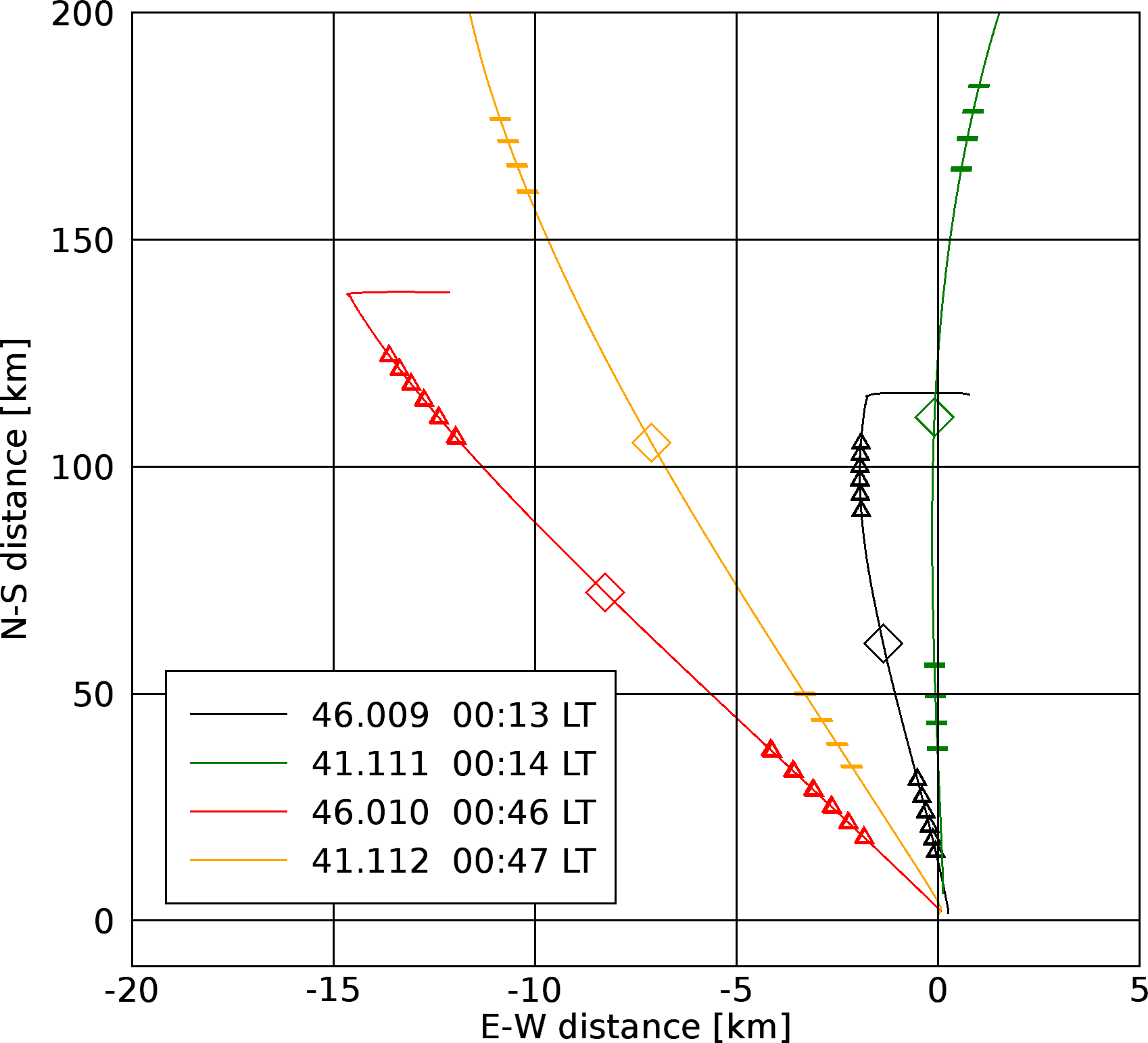
Figure 1Horizontal projection of the four sounding rocket trajectories. The triangles mark altitudes 70 to 120 km in 10 km steps on upleg and downleg for the instrumented payloads (MTeX 46.009 and 46.010), and the dashes mark altitudes 90 to 120 km for the chemical tracer payloads (MIST 41.111 and 41.112). The diamonds mark the apogees.
Figure 1 illustrates the horizontal separation of all four flights. Note the different east–west and north–south scales. The black and red triangles mark the four sets of CONE measurements between 70 and 120 km. Green and orange marks show the location of the tracer releases between 90 and 120 km. For the MTeX flights the altitude of 70 km was reached after 65 s on the upleg and 339 s on the downleg. The launch azimuth was 0.0∘ (due north) and 0.6∘ for 46.009 and 46.010, respectively. The horizontal separation between 70 km upleg and 70 km downleg was about 88 km for 46.009 and 105 km for 46.010. As can be seen in the figure, the flights of the second salvo veered slightly westward, but the difference is small in comparison to the extent in the north–south direction.
2.2 CONE instrument, neutral densities and fluctuations
The CONE instrument is a spherical hot-cathode ionization gauge designed for pressures up to ∼1 mbar and has been flown over 20 times since the 1990s (Giebeler et al., 1993; Rapp et al., 2001), including on four previous NASA payloads (Lehmacher et al., 2006, 2011). Neutral air is ionized by electron impact and the collected ion current is the primary measurement signal. A sketch of the CONE instrument can be found in Rapp et al. (2001). Here we include specific details of our methodology, which is similar to the standard procedure (Rapp et al., 2001; Strelnikov et al., 2003). We want to stress the fact, that this is the first application of individual CONE instruments measuring in the ram direction on both upleg and downleg. This will help us in assessing the significance of observed differences in the mesospheric structure.
The ion current varies between ∼1 and 8000 nA, for altitudes from 130 to 65 km, and is measured by a five-step, auto-ranging electrometer with 16-bit digitization and 5208 samples per second (or ∼0.2 m at 1000 m s−1). The electron emission current from the filament is kept constant at 14 µA, so that the ion current is roughly proportional to the neutral density. Small deviations from linear behavior were recorded in a calibration vacuum chamber using an MKS Baratron capacitance manometer with mbar accuracy. We calculated the ion currents using the voltage output for each electrometer range calibrated with a Keithley 261 Picoampere source (Guido Krein, personal communication, 2017). We removed a few data spikes due to range switching and adjusted the voltage offsets in each range to generate a continuous profile for the ion current. Figure 2 shows the ion currents versus altitude for all four profiles.
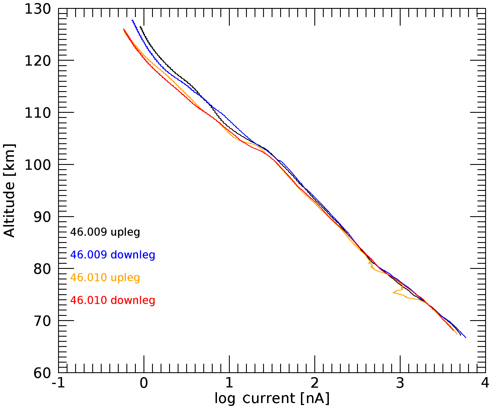
Figure 2Four profiles of ion currents observed during the MTeX flights. Each pair of upleg and downleg profiles was obtained with a single CONE instrument.
The graph clearly shows that the sensitivity of the two CONE ionization gauges is different at lower currents corresponding to altitudes above 100 km, while the variation is very small between 70 and 90 km, indicating similar sensitivity for both gauges. Therefore, we expect similar densities for all four profiles at lower altitudes. During the upleg of 46.010 (orange profile), we observed strong disturbances of the ion current near 75 and 80 km, and associated disturbances of the emission current (not shown).
The cause of these disturbances is not understood, but simultaneous observations from a small, sensitive three-axis accelerometer included in the MTeX payload provide indirect evidence of the the existence of a large mesospheric wind. Here we include the main results of this new diagnostic tool. We have deferred the technical details of the accelerometer analysis and comparison with CONE data to the Appendix.
The accelerometer was mounted close the payload spin axis (z) near the center of gravity and observed how the residual drag acceleration decreased with exponentially decreasing density. For flight 41.010, near 75 km, the average z component of the acceleration was 3.7 and 3.3 mg on the upleg and downleg, respectively (Fig. A1). A direct Monte Carlo simulation (DSMC) of the supersonic flow using the velocity, density and temperature conditions for this flight yielded a drag force of ∼7.2 N at 75 km, corresponding to a drag acceleration of ∼4.0 mg, in reasonable agreement with the observations.
The perturbations in the CONE measurement, only on the upleg of 41.010, were unexpected and unprecedented for this instrument. Upon close inspection, we noticed coincident small changes in acceleration of ∼0.5 mg near 75 km. No ACS maneuver or other payload event occurred at this time that could have perturbed both measurements, and the angle-of-attack analysis performed by NASA Wallops Flight Facility showed no deviation; therefore, we suggest that a large wind may have altered the drag force. We performed DSMC simulations adding winds and found that a horizontal wind of 100 m s−1, which reduces the ram flow by 30 m s−1, can indeed reduce the drag force and the relevant acceleration component by 5 % or 0.2 mg.
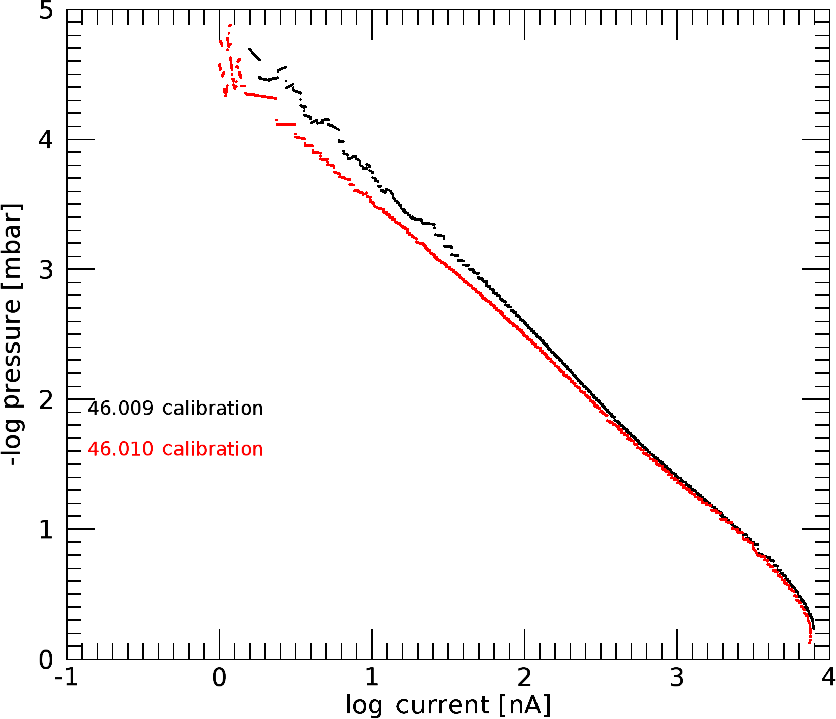
Figure 3Ion currents observed during laboratory calibrations of the two CONE sensors. Irregularities at pressures below 10−3 mbar in one of the profiles are due to irregularities in the gas flow into the chamber and can be ignored.
The purpose of the sensor calibration is to correct for the nonlinear variation between pressure and ion current and to account for differences between individual instruments. The calibration for the two CONE ionization gauges is shown in Fig. 3. The gauge used for flight 46.009 was more sensitive above 10−2 mbar, consistent with the current measurements observed in the flights (Fig. 2). Before applying the calibration information, we reduced the original data rate of 5208 samples per seconds by a factor of 100 and applied a low pass filter to suppress a small modulation with the spin rate of 2 Hz. In order to model the calibration curves, we used a combination of a linear function up to 10−2 mbar and three Gaussians for higher pressures and converted the currents to pressures and densities. The parameters of the calibration functions were tuned to match a common density profile below ∼80 km, where atmospheric conditions are most stable over the duration of the experiment.
After applying the calibration, the densities obtained correspond to what is measured inside the CONE ionization volume, and these values are larger than the densities in the free atmosphere due to compression effects in the supersonic flow (Rapp et al., 2001). We apply an aerodynamic “ram” correction that was determined using DSMC calculations for zero angle-of-attack and altitudes between 120 and 70 km. These “ram factors” vary between 1.6 and 2.6 and were originally calculated for a previous sounding rocket experiment carrying the CONE sensor (Lehmacher et al., 2006). Although the MTeX flights achieved a higher apogee (156 vs. 135 km) and higher Mach numbers (M∼4.5 vs. 4.0) than the earlier flight, we find that extrapolating these ram factors works well for our flights. Although the ram factors for the CONE sensor are relatively constant at small and moderate angles-of-attack (Rapp et al., 2001), MTeX was the first experiment where the angle-of-attack for CONE was very close to zero due to the use of an attitude control system. Figure 4 shows the densities after the ram correction, which closely agree with NRLMSISE-00 (hereafter simply MSIS) model densities (Picone et al., 2002). Large wavelike deviations above 100 km, that could already be seen in the current profiles, are significant features in the lower thermosphere.
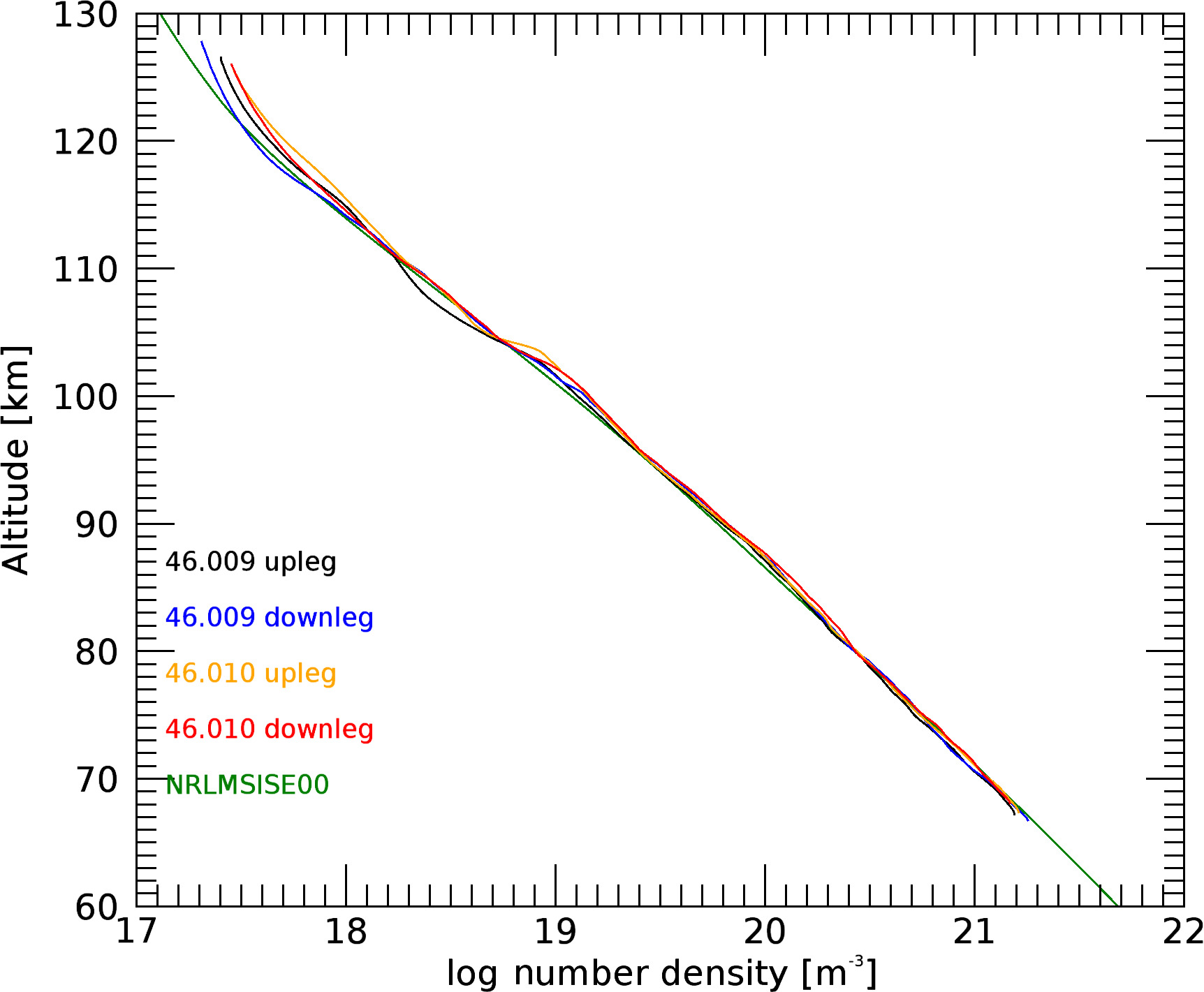
Figure 4Neutral number densities for four profiles after calibration and ram correction. The four profiles agree now for all altitudes, but display significant variability above 100 km.
The temperature profiles T(z) are obtained by integrating the density profile from low to high densities and using the start temperature T0(z) at 115 km taken from the MSIS model. Only the relative density profile n(z)∕n0(z) matters and the uncertainty in the start temperatures vanishes after one to two scale heights (Rapp et al., 2001).
Finally, we calculate the buoyancy frequency as
Temperature profiles and buoyancy frequencies are discussed in the next section.
Our method to calculate atmospheric densities using calibration data and ram correction follows the standard procedure (Rapp et al., 2001) and is independent from external data sets (except the start temperature). An alternative method is to use the relative density profile from the nightly averaged Rayleigh lidar signal to normalize the CONE current data, which results in smoother density gradients and temperatures (Triplett et al., 2018).
The open geometry of the CONE ionization gauge aids in the observation of very small neutral density fluctuations (<0.1 %) which are neutral, inert, scalar tracers of turbulence (Lübken et al., 1993). The assumptions and principal methodology of the spectral analysis have been described by Lübken et al. (1993) and rely on observing the transition from inertial to viscous scales in the density fluctuation spectra (Kolmogorov, 1941), characterized by the turbulent inner-scale ℓ0 based on the Heisenberg (1948) model.
While the energy dissipation rate ϵ (which is determined from ℓ) can vary over several orders of magnitude, the kinematic viscosity increases exponentially with the scale height. Typical inner scales in the mesosphere and lower thermosphere are 10–50 m, which requires measurements at meter-scale resolution to identify the viscous subrange.
As noted already, MTeX was the first experiment with the CONE instrument mounted on an actively stabilized payload, and aligned closely to the velocity vector (angle-of-attack close to zero). The spin rate was actively reduced to about 2 Hz. It is well known that small asymmetries in the supersonic flow around the ion gauge lead to modulations of the current signal at the spin frequency and higher harmonics (Hillert et al., 1994; Strelnikov et al., 2003). At 1000 m s−1, the payload has moved 500 m during one spin period, which means that the much smaller inner scale is easier to detect at the low spin rate than at common, higher spin rates, e.g., 6 Hz. Also, at larger angles-of-attack, the spin modulation and higher harmonics cause major interference with the turbulence signal (Lehmacher et al., 2011); therefore, the alignment was important in obtaining good turbulence data.
The time series to be analyzed are relative fluctuations of the ion current I(t)∕I0 (identical to relative neutral density fluctuations n(t)∕n0 over short intervals), which are determined by subtracting and dividing by a 1000-point (0.2 s) running average. Figure 5 shows as an example the relative fluctuations for the upleg of flight 46.009.
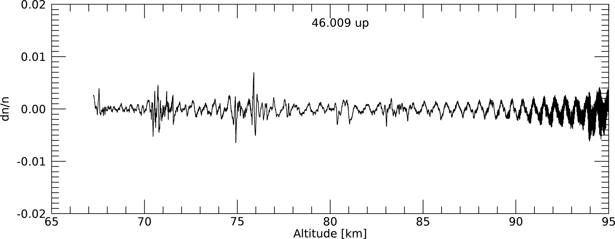
Two regions of neutral density fluctuations can immediately be recognized around 71 and 76 km altitude. Note that the level of fluctuations is much less than 0.01 (1 %). A small spin modulation becomes more prominent above 85 km. The increasing noise above 90 km was caused by interference from the voltage sweeps of the Langmuir probe on one of the booms (Collins et al., 2015). Turbulent fluctuations, which have larger scale sizes (hundreds of meters) at higher altitudes, can easily be distinguished from these small-scale, regular perturbations.
We have used the wavelet method first applied to CONE data by Strelnikov et al. (2003), which allows for a finer localization of turbulence layers. The alternative method of calculating fast Fourier transform (FFT) spectra over 1 km or larger intervals can lose some detail in the lower mesosphere, but is better at capturing larger scales in the upper mesosphere. An example turbulence spectrum from the lower mesosphere is shown in Fig. 6.
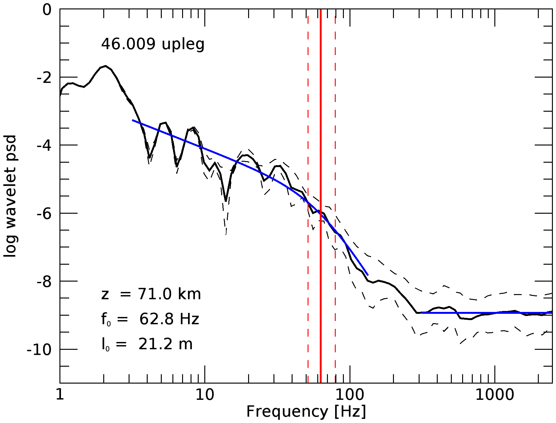
Figure 6Example of wavelet spectrum of turbulent fluctuations. The blue curve is a best fit of a theoretical spectrum including the transition from the inertial subrange to the viscous subrange. For details see text.
Individual wavelet spectra were averaged over 100 m intervals. The thick black line is such an averaged wavelet spectrum for the interval 71.0 to 71.1 km. The blue line is the least-square fit of a Kolmogorov–Heisenberg spectrum for stationary, homogeneous, isotropic turbulence with slopes and −7 in the inertial and viscous subranges, respectively. Turbulent spectra were fitted if the data displayed a slope of −5 or steeper in the frequency range between 31.6 and 316 Hz, which is where the viscous subrange can be found. Additionally, some spectra were eliminated if they did not show an inertial subrange with slope . The red line in the figure indicates the frequency at the fitted inner scale, in this case 21 m. Frequency and scale size are converted via the payload velocity, . Spectra with one standard deviation above and below (dashed lines) were fitted for an error estimate of f0, l0, and ϵ. In this example the lower estimate was 17 m and the upper estimate 27 m. Since the energy dissipation rate depends on the fourth power of the inner scale, lower, middle, and upper estimates are 0.68, 1.5, and 3.9 mW kg−1, values that are in line with previous measurements of turbulence in winter at high latitudes (Lübken, 1997; Lübken et al., 1993).
We will discuss temperature, buoyancy frequency and turbulence results in Sect. 3.
2.3 Chemical tracers
Both MTeX launches were closely followed by two MIST payloads for wind and turbulence measurements in the lower thermosphere. TMA trails were released on the upleg and downleg between ∼80 and 150 km. Cameras for ground-based photography of the trail were located at Poker Flat, Coldfoot (67.25∘ N, 150.15∘ W), and Toolik Lake (68.63∘ N, 149.60∘ W). For a review of the technique see Larsen (2002). Typical errors of horizontal wind components are 5–10 m s−1. In the next section, we show wind profiles calculated from the upleg trails and examples of trail structures as they relate to the observed winds and temperatures.
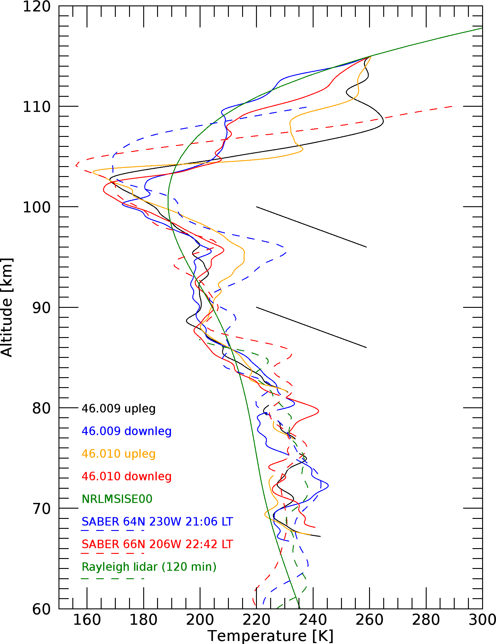
Figure 7Temperature profiles (solid lines) derived from densities in Fig. 4. Start values at 115 km were chosen from MSIS (green line). Individual SABER temperature profiles (blue and red dashed lines) obtained during that night in this area show good agreement with the general temperature structure. The legend lists times and tangent point location for these profiles. The Rayleigh lidar profile was obtained by integrating data from 23:30 to 01:30 LT (green dashed line). The two straight solid lines indicate the adiabatic gradient of −9.7 K km−1.
3.1 Temperatures
Figure 7 shows all four temperature profiles derived from CONE densities combined in one plot. The start temperature is chosen from the MSIS profile at 115 km; given the large variations around 105 km, we estimate an uncertainty of 30 K at 115 km, which is larger than the instrumental error of ∼3 K, and decreases exponentially towards lower altitudes (Rapp et al., 2001). The four profiles are similar, which is expected given the moderate horizontal and temporal separation (see Fig. 1). (For the upleg of 46.010 (orange), we interpolated the densities logarithmically in the two regions, where the CONE currents were disturbed. These regions are shown as gaps in the orange profile.)
Characterizing the large features of the profile, we observe a relatively warm winter mesosphere up to 80 km, a quasi-adiabatic region between 80 and 88 km, another stable region up to 95 km, followed by a second quasi-adiabatic region up to the mesopause at 170 K and 102 km. The two bottommost regions agree well with the Rayleigh lidar temperatures (Triplett et al., 2018). The lower thermosphere is highly structured; the upleg profiles have temperature excursions up to 60 K warmer than MSIS between 105 and 110 km. The mesopause is markedly colder than MSIS, a feature that we also observed during an earlier winter experiment together with significant large-scale, long-period wave activity (Lehmacher et al., 2011). In the graph, we included two SABER temperature profiles with tangent points closest to the rocket observations. The distances between tangent points and rocket measurements was approximately 840 and 310 km for the profiles obtained at 21:06 and 22:42 LT, respectively. SABER stands for Sounding of the Atmosphere using Broadband Emission Radiometry and is an instrument on the Thermosphere Ionosphere Mesosphere Energetics Dynamics satellite (TIMED) in operation since 2002. Despite a very different technique and sampling geometry for a satellite limb sounder, both SABER profiles show remarkably similar structures: a distinct and relatively cold mesopause, and two quasi-adiabatic regions bracketing a stable region.
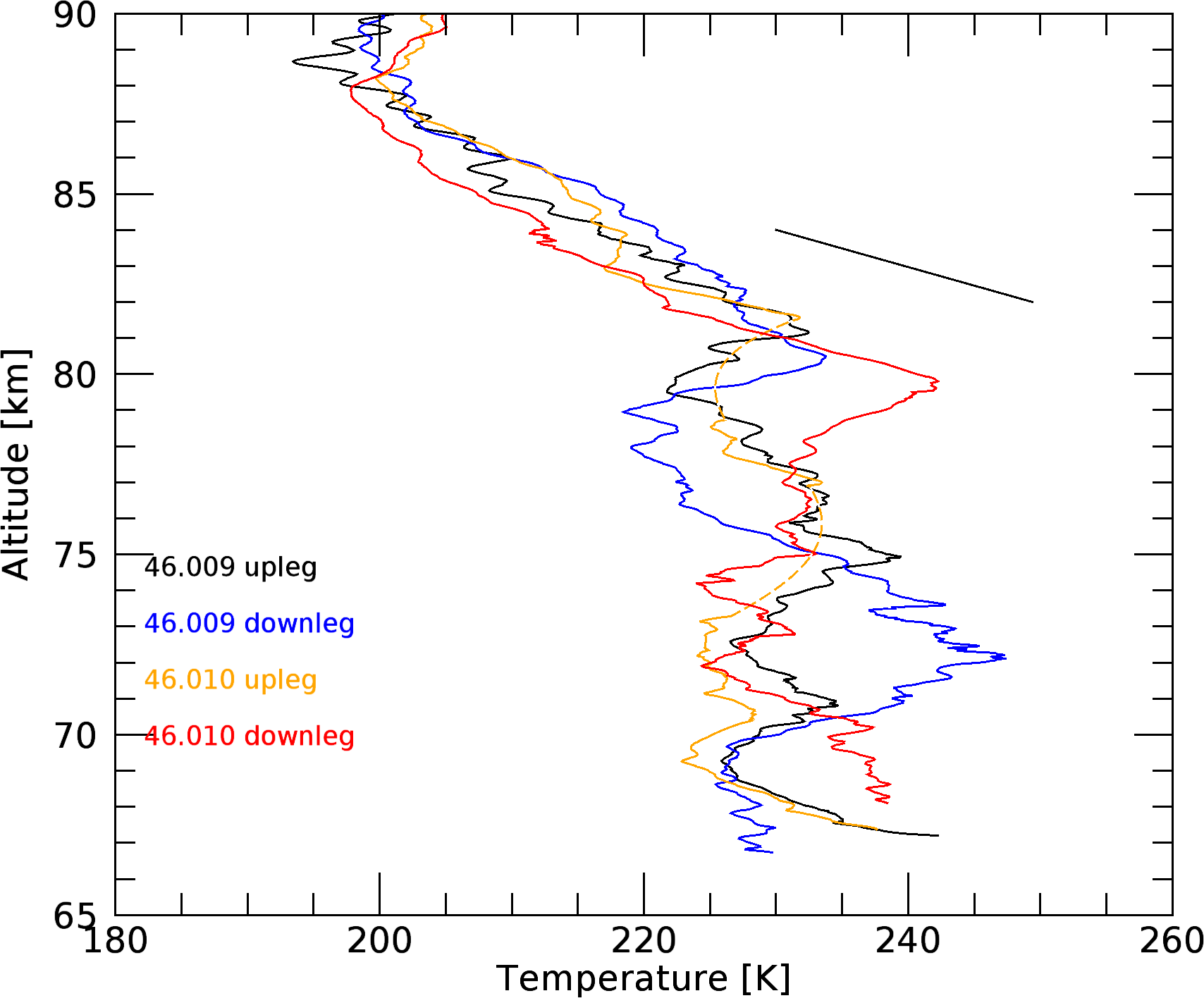
Figure 8Detail of temperature profiles in the lower mesosphere. Same data as in Fig. 7, but unfiltered to emphasize fine structure. The regular modulations above 80 km in the black profile are due to the payload spin.
Figure 8 shows details of the CONE temperature profiles. For this plot, the in situ data have not been low-pass filtered; therefore, flight 46.009 shows some spin modulation that could also be seen in Fig. 5. On the other hand, temperature fluctuations below 80 km are a clear indication of the sub-kilometer dynamics in the mesosphere that only in situ instruments can detect. The 46.009 downleg profile (blue) differs significantly from the other profiles near 72 km, while the upleg profiles, which were closest together, agree well (if we ignore the interpolated altitude intervals). Consecutive lidar profiles showed that the wave activity, based on the lidar temperatures during the night, was relatively weak and at the time of the launches only small inversion layers near 61 and 70 km were present over the launch site. The nightly lidar average also reproduces the strongly negative temperature gradient above 80 km (Triplett et al., 2018).
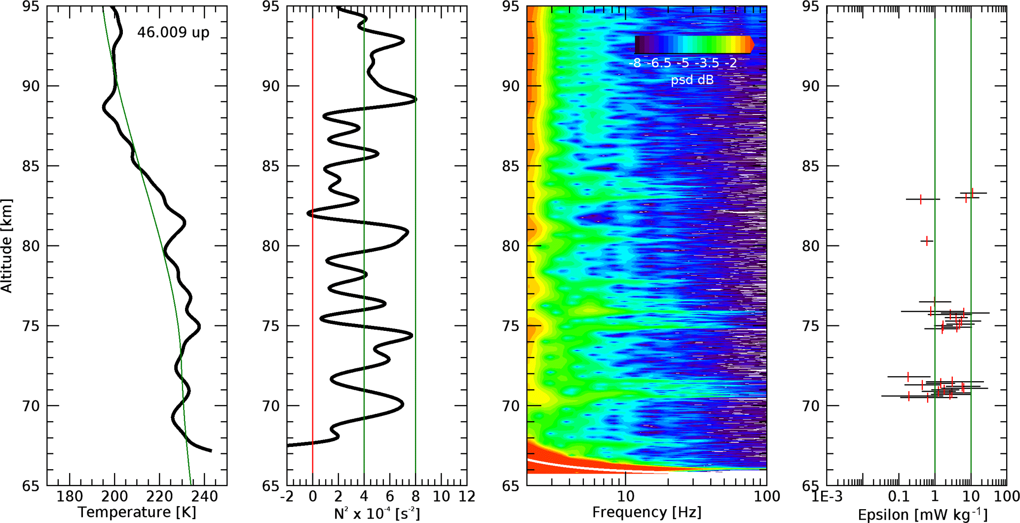
Figure 9Temperature profile, buoyancy frequency, wavelet spectra of neutral density fluctuations, and turbulent energy dissipation rates for flight 46.009 upleg. For details see text.
3.2 Buoyancy frequency and turbulence
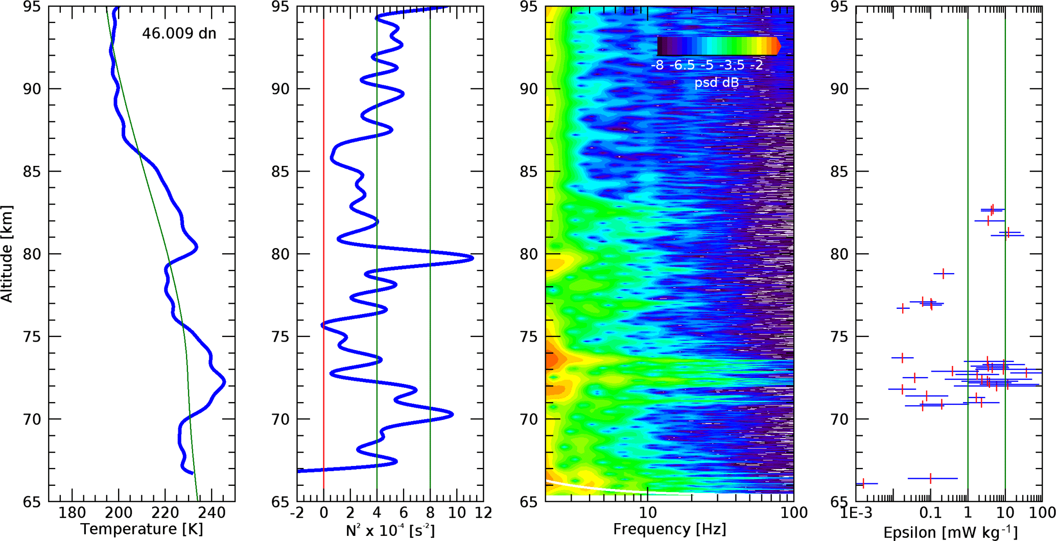
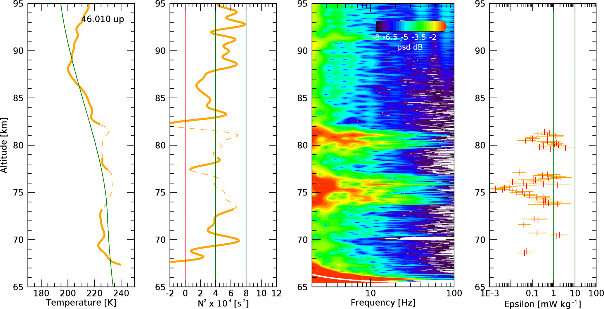
Figures 9–12 compare the temperature and turbulence structure side by side for each profile. The green line is an MSIS model profile. The second panel shows the square of the buoyancy frequency N2 derived from the temperature profiles. It is important to note that the N2 profile is quite robust since the locations of stable and unstable regions are independent of the absolute temperature. The red line at N2=0 corresponds to the adiabatic temperature gradient and serves as a guide for instability; the two green lines at and are chosen as arbitrary values for average and stable conditions. Most of our data are are contained between these values. The third panel shows the spectrogram of the global wavelet spectra of the neutral density fluctuations at 100 m resolution, as described above. Above 85 km, signal modulations with the spin frequency and harmonics at 2, 4 and 6 Hz become significant, as can already be seen in Figs. 5 and 6. A white line near the bottom indicates the “cone of influence”, where wavelet power cannot be estimated (Torrence and Compo, 1998). The fourth panel shows the energy dissipation rates ϵ derived for 100 m intervals with upper and lower estimates, as explained in Sect. 2.
The first profile was obtained on the upleg of flight 46.009. Two distinct layers of turbulence were observed centered around 71 and 75 km, respectively. Energy dissipation rates in these layers ranged from 0.18 to 6.4 mW kg−1 and the median values in the lower and upper layer were 1.5 and 2.7 mW kg−1, respectively. The lower layer is mostly above a small local temperature maximum at 71 km associated with an inversion layer. The upper layer is near a smaller local temperature maximum. A second inversion layer was observed near 80 km with a temperature maximum near 81.5 km. There are density fluctuations between 83 and 84 km with smaller cut-off frequencies (larger inner scales). A few spectra could be fitted with energy dissipation rates of up to 7 and 11 mW kg−1.
The second profile was observed on the downleg of flight 46.009, 70 km north of the upleg profile. The temperature profile is significantly different in the lower mesosphere and has a broad maximum at 72.5 km associated with a deep turbulence enhanced layer. The maximum energy dissipation rate is found at 72.8 km with 36 mW kg−1, slightly above the temperature maximum. The median value for the entire layer is 2.2 mW kg−1. It appears that the two regions of turbulence generation observed on the upleg are merged at this location; however, this cannot be verified without additional observations at intermediate locations. The inversion layer at higher altitudes is very distinct in this profile with a clear maximum of the buoyancy frequency near 80 km, slightly lower that on the upleg. Again, there was a less distinct layer between 81 and 83 km, with values up to 12 mW kg−1.
The third profile was obtained on the upleg of flight 46.010. Its location was very close to the first profile and the measurement occurred 33 min later. As explained above, we do not have a complete density and temperature profile due to the anomaly of the CONE sensor, and the interpolated regions are marked with dashed lines. However, it can be assumed that the temperature profile did not change dramatically compared to the first profile, as can be seen below 73 km and also above 82 km where the measurements were undisturbed. This is also confirmed by the series of Rayleigh lidar profiles. With this caveat in mind, we did the wavelet analysis of the ion current fluctuations in the perturbed regions and found that the spectra conformed with our turbulence model, although the fluctuations were much amplified in the perturbed regions, as can be seen from the red contours in the spectral plot. Compared to the 46.009 upleg, the turbulent layer near 70 km had weakened or moved by advection, although there is still a thin layer present at 70.5 km with 1.8 mW kg−1. These data were not affected by the anomaly. The layer around 75 km from the 46.009 upleg may have expanded; it stretches now from 74 and 77 km. The dissipation rates are slightly smaller and reach only 2.0 mW kg−1. The biggest difference in the 46.009 upleg is observed near 80 to 81 km, where no turbulence was observed 33 min earlier. On the 46.010 upleg, this region exhibits strong fluctuations with inner scales corresponding to energy dissipation rates up to 1.3 mW kg−1. The temperatures in the undisturbed region near 82 km suggest super-adiabatic conditions. Further support for strong mixing in this region comes from the sodium densities and mixing ratios observed by lidar (Triplett et al., 2018). Low sodium density air was mixed upward in a major overturning event and extended from 81 to 88 km during the two flights. This agrees strikingly well with the quasi-adiabatic region observed in all four in situ profiles.
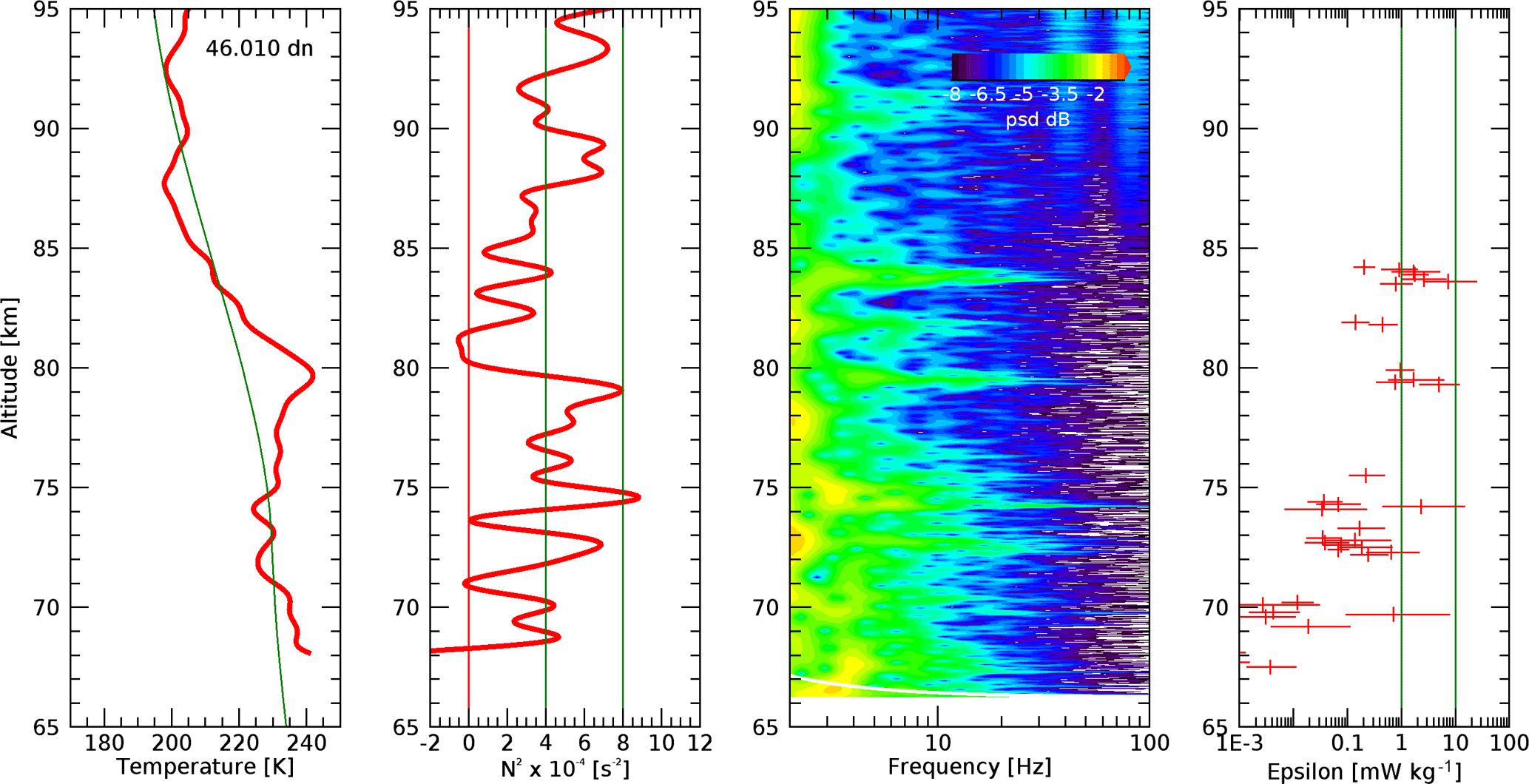
The last profile was obtained on the 46.010 downleg, about 10 km west of the first downleg. The temperature profile agrees in many details with the other three profiles, most significantly, the local maximum near 80 km below a deep layer with low static stability, as just discussed. At the lower altitudes we find very weak turbulence in several narrow layers near 70, 72.5, and 74 km, mostly associated with stable regions of the atmosphere. The largest value is 2.3 mW kg−1 at 74.2 km in a very thin layer. The region of turbulence in the lower mesosphere is broadly consistent with the observation from the 46.009 downleg, but the intensity level is weaker. In contrast to the earlier downleg profile, two strong, but narrow layers were observed near 80 and 84 km with maximum epsilon values of 4.0 and 7.3 mW kg−1. The lower of these layers coincides with the local temperature maximum near 80 km, the upper with local stability maximum near 84 km.
In summary, and perhaps not surprisingly, we observe strong similarities in the large-scale temperature and stratification structure, but great variability in the altitude, thickness, and strength of the fluctuation layers. It is important to note that, common in all four profiles, turbulent spectra are found mostly in the more stratified region below 80 km, while fluctuations and turbulence are largely absent in the well-mixed layer above.
3.3 Neutral winds, Richardson number, and trail structure
Figure 13 shows the zonal, meridional and total horizontal wind profiles obtained during the upleg releases as red, blue and black lines, respectively. Common features are an extreme westward zonal wind shear near 110 km and strong westward winds above. Below 105 km, winds were smaller and relatively constant. Above 110 km, the winds significantly changed between the first and second flights; the zonal component weakened and the meridional component shifted southward. The flights occurred under moderately active conditions and a bright auroral arc. High southwestward wind speeds of 200 m s−1 above an extreme zonal wind shear were also observed during the ARIA II experiment under moderate to high geomagnetic activity (Larsen et al., 1997).

Another presentation of the wind components are the hodographs in Fig. 14. Symbols mark altitudes in 1 km steps; the big, filled circles mark 90, 100, 110, 120 and 130 km. The lowest altitudes start on the right and the wind vector rotates clockwise with increasing altitude. Particularly, MIST-2 showed a consistent rotation up to 110 km, typical of a tidal or inertia-gravity wave, but stretched out by the strong westward shear. A similar wave without any additional shear was observed during geomagnetically very quiet conditions (Lehmacher et al., 2011). While in both cases large-scale gravity wave activity was observed, we point out that in addition to the wind shear also the temperature profiles were more perturbed than in the very quiet case.
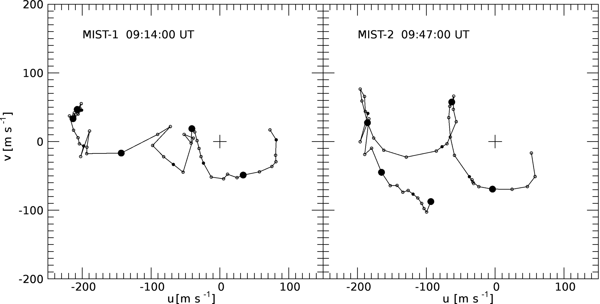
Figure 14Hodograph projections of the horizontal wind. The lowest altitudes start on the right at positive zonal winds. Small open circles are drawn every 1 km and large filled circles every 10 km. The first large circle is at 90 km. The cross marks the origin (zero wind).
The simultaneous measurements of temperatures with the CONE instrument and winds with the chemical tracer technique allow the calculation of Richardson numbers as an index for instability (Howard, 1961; Miles, 1961) in the turbopause region. This is only the second experiment for which this combination of measurements was available. We interpolated CONE upleg temperatures in 1 km intervals to match the upleg wind data and calculated the Richardson number as
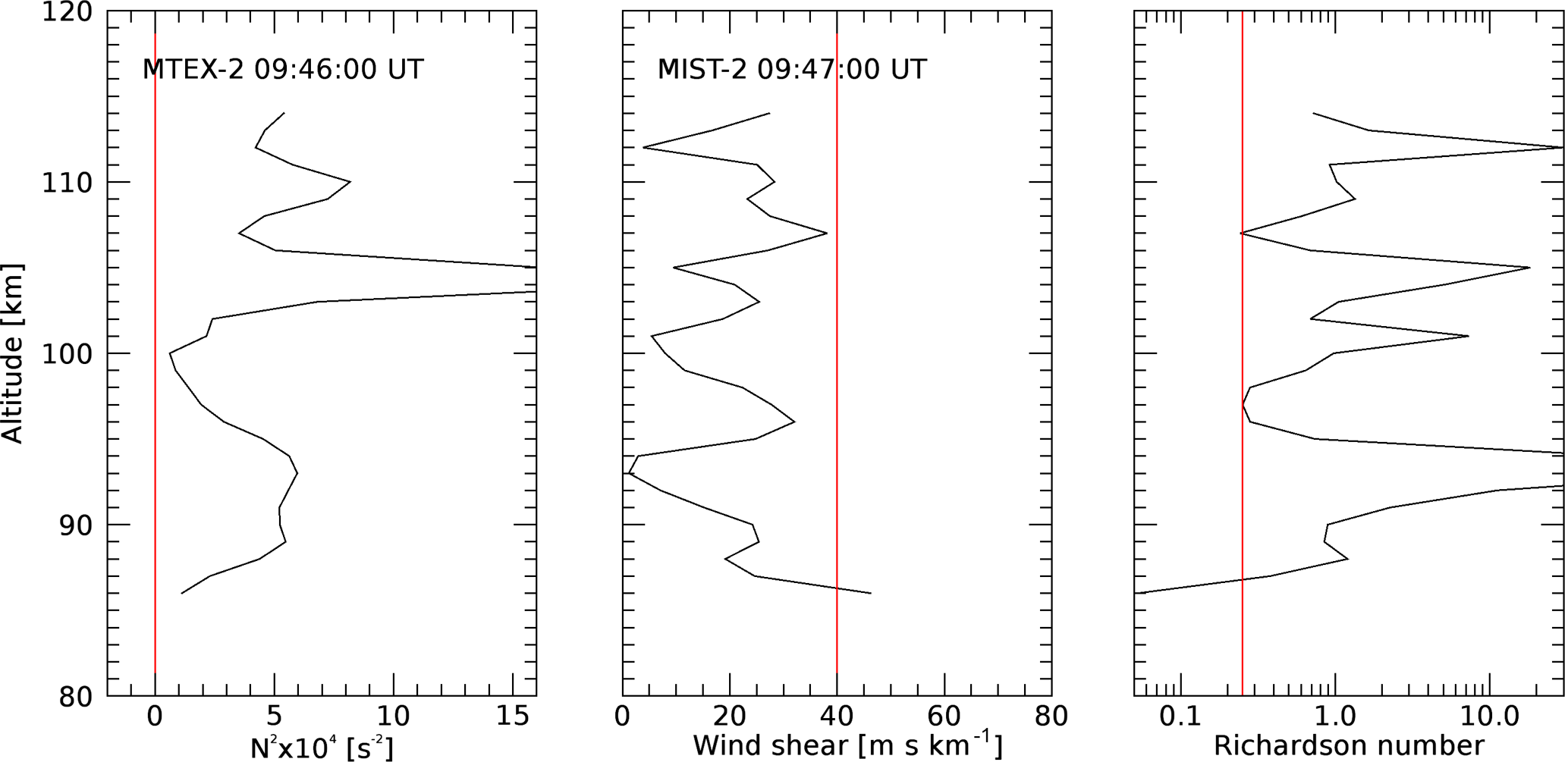
In Figs. 15 and 16 we show profiles of buoyancy frequency, horizontal wind shear, and Richardson number at altitudes, where we have simultaneous temperature and wind data. For the first salvo, we find a minimum in the Richardson number of less than 0.1 at 110 km. At this altitude, the buoyancy frequency was unusually low, paired with an extreme wind shear. For the second salvo, similar conditions existed at 107 km. All four temperature profiles (Fig. 7) showed regions of warmer temperatures in the lower thermosphere between 102 and 110 km, most prominently in the upleg profiles. We point out that we did not find small-scale density fluctuations in this overlap region, nor have other coincident observations of energy dissipation rates that could be related to the regions of low Richardson numbers.
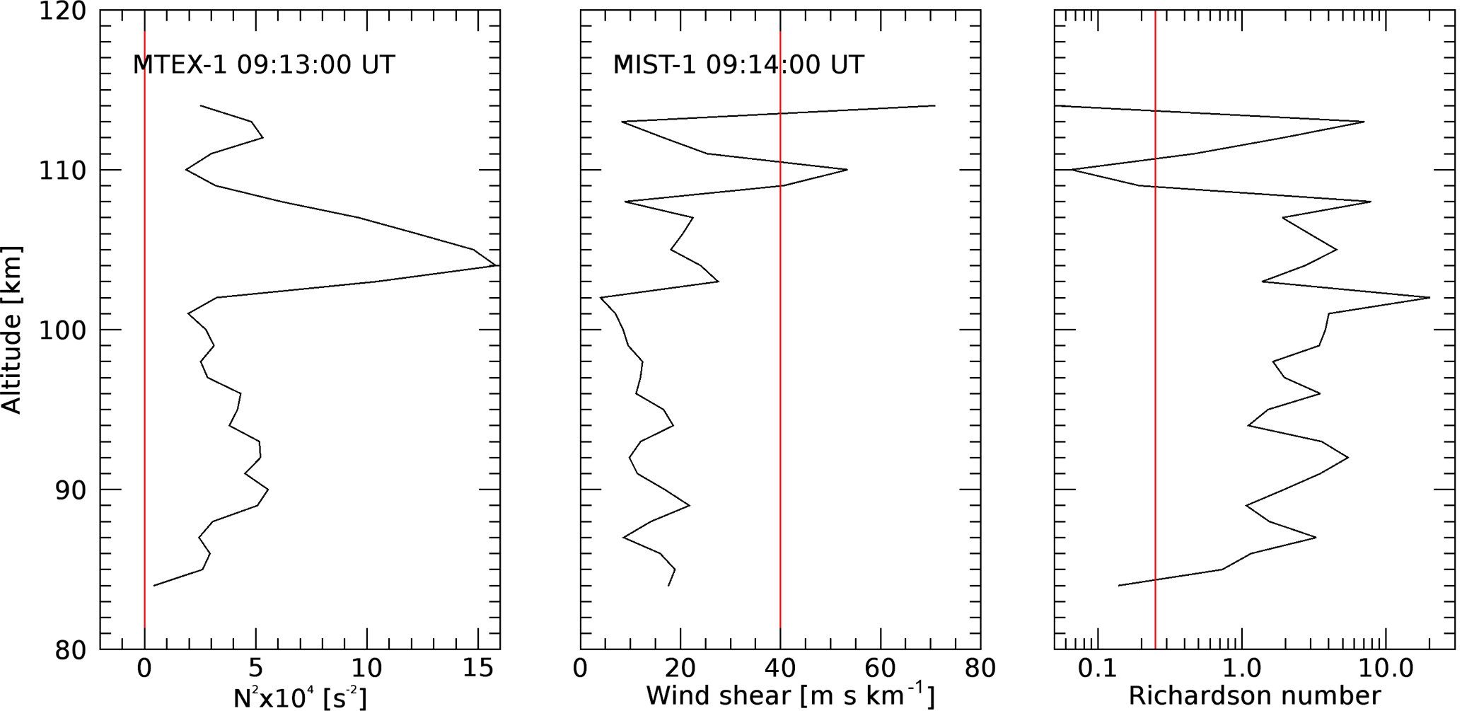
Figure 15Buoyancy frequency from CONE upleg temperatures, horizontal wind shears from TMA winds, and Richardson numbers for the first salvo. The red line in the right panel indicates Ri=0.25.
The extreme wind shear is also directly visible in the images of the puffed TMA trails. Figure 17 shows the upleg trail viewed from the north from Toolik Lake (68.63∘ N, 149.60∘ W) (a) and from below from Poker Flat (b). About 70 s after the release, the chemiluminescent material at 110 km was already stretched out (shown by the red arrows). In this region, above the turbopause, no small-scale irregularities were visible. The Reynolds number is small in this region and the flow remains laminar (Blamont and de Jager, 1961).
Below ∼103 km, the trails often develop billows of large and small sizes due to atmospheric turbulence (Blamont and de Jager, 1961; Roberts and Larsen, 2014). A very clear example can be seen in both downleg trails as viewed again from north from Toolik Lake (Fig. 18). These images were taken 190 s after TMA was released at 100 km on the downleg. The trails between 95 and 100 km (red arrows) appear as vertical billowing columns with a defined top. The lower part of the trail is stretched to the left in the images due to predominantly eastward winds (see Fig. 14). The temperature structure measured 50 km further south shows a quasi-adiabatic lapse rate between 95 and 100 km and a very stable layer above (see Fig. 7). Considering both TMA images and temperature structure, this suggests the presence of a convection layer just below the mesopause. The region of low stability (N2∼0) may include super-adiabatic conditions and cause the acceleration and large vertical displacements of air parcels. Modeling results show furthermore that such regions are less likely a location of strong wave breaking and turbulence generation, since medium-scale waves are evanescent in these regions (Jonathan Snively, personal communication, 2018). Roberts and Larsen (2014) used the entire downleg trail below the turbopause to determine the structure function coefficient as a function of scale size, while the large-scale temperature structure was unknown. Our case presents an opportunity to study the evolution of the structure function under known stability conditions.
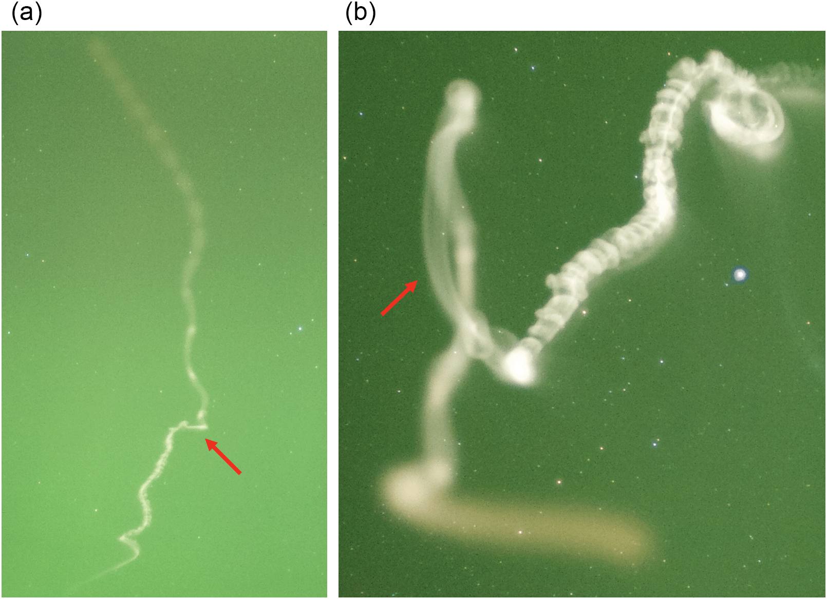
Figure 17Photographs of the MIST-1 upleg trail from Toolik Lake (a) and Poker Flat (b) at 09:16:59 UT. The 110 km region is located where the trail is marked by the arrows.
The MTeX experiment was the first time that four profiles of in situ neutral turbulence and background temperature were obtained close together in time and space. While this is still a very small sample of the turbulent flow field, it allows a limited comparison with high-resolution multi-scale gravity wave breaking simulations.

Figure 18Photographs of the MIST-1 (a) and MIST-2 (b) downleg trail from Toolik Lake (a) taken at 09:23:24 and 09:56:24 UT, respectively. The arrows indicate the bottom and top of the quasi-adiabatic layer near 95 and 100 km, respectively.
Fritts et al. (2018a, b) presented cases of the interaction between a small-scale monochromatic gravity wave (λx=20 km, λz=20 or 40 km) and a MIL, which was centered at 80 km and spanned about 20 km. The numerical simulations showed that the interaction was relatively weak and did not create layers of instability or weakened stability several kilometers deep.
During our experiment, we did not encounter a large MIL of the type set as the temperature background in the simulation. However, the mesosphere was on average stable below 80 km and very weakly stable or quasi-adiabatic between 80 and 88 km. Almost all of our turbulence layers were observed in the more stable region below 80 km. The perturbations in stability due to GW interactions resemble the individual N2(z) profiles shown by Fritts et al. (2018b) in their Fig. 13. Our upleg and downleg results show little relation; patchiness is expected for turbulence over this spatial domain, and is also found in the multi-scale simulations. We also found significant differences in the turbulence strength and layer distribution between the first and second flights. Numerical simulations of gravity wave breaking show significant evolution over 30 min (∼five buoyancy periods).
Comparing values for the energy dissipation rate, the statistics of winter turbulence measurements obtained at Andøya (Lübken, 1997; Lübken et al., 1993) was recently extended and updated by Szewczyk (2015). Average energy dissipation rates increase continuously from 1 mW kg−1 at 70 km to 10 mW kg−1 at 80 km, up to a maximum of 50 mW kg−1 at 90 km, while the total variability envelopes cover almost 4 orders of magnitude. Our values fall well within this range; however, the absence of significant turbulence above 80 km seems unusual during our flights. As mentioned earlier, Triplett et al. (2018) found that gravity wave activity in the 40–50 km region during this period was extremely low and suggested that this may have contributed to reduced gravity wave breaking and turbulence activity in the upper mesosphere.
In an earlier experiment from Poker Flat, fluctuation activity was small in the lower mesosphere, despite a prominent mesospheric inversion layer at 70 to 75 km (Collins et al., 2011; Lehmacher et al., 2011). An overturning event in the sodium layer coincident with a near-adiabatic layer between 75 and 80 km suggested that it may have been accompanied by strong downward turbulent heat flux (Collins et al., 2011); however, the new simulations by Fritts et al. (2018b) did not produce significant heat fluxes above the temperature inversion. On the other hand, a turbulent layer was observed in this earlier experiment between 88 and 90 km, with energy dissipation rates up to 30 mW kg−1, observed in neutral and electron fluctuations.
Another winter case study was presented by Szewczyk et al. (2013). A strong temperature inversion between 86 and 89 km and quasi-adiabatic layer between 89 and 91 km was strongly turbulent, especially in the adiabatic region. It was concluded that gravity wave breaking and turbulent heating was creating or maintaining the inversion layer, also at odds with the recent modeling results by Fritts et al. (2018b). Previously, Liu et al. (2000) had carried out a 2-D modeling study of gravity wave–tidal interaction that produced extremely high GW heat fluxes and adiabatic gradients. The model was set up to test the hypothesis that this type of wave–wave interaction can generate and maintain MILs. The model results suggested that direct turbulent energy dissipation was small compared to the overall heating rates obtained in the model.
Lehmacher and Lübken (1995) reported the results of a mid-latitude study of turbulence generation in a deep, partially super-adiabatic layer between 75 and 80 km. This suggests that small-scale turbulence can be important in initial gravity wave breaking and mixing in the mesosphere, but once the layer is well mixed, turbulent fluctuations are largely absent. It is true that for strictly vertical adiabatic motions on top of an adiabatic background, i.e., N2=0, density fluctuations cannot be observed, since (Lübken, 1992)
Szewczyk (2015) presented a statistical study of a large number of in situ neutral turbulence profiles, which showed that mesospheric turbulent density fluctuations have a normal distribution over buoyancy frequency with a maximum near K km−1. However, there is still a significant number of cases, where dT∕dz is between −9 and −11 K km−1.
A recent sounding rocket flight from Andøya was equipped with two CONE instruments to provide measurements on the upleg and downleg (Strelnikov et al., 2017). This was in summer, however, when the temperature and turbulence structure is different than in winter (Lübken et al., 1993). In this case, a relatively large variability in temperatures was observed between the upleg and downleg portions of the flight, which were separated by 41 km at 70 km altitude. Other observations, such as VHF radar echoes and winds, also showed large horizontal variability. It was suggested that a gravity wave with 30 km horizontal wavelength could have modulated the temperature field and associated turbulence generation.
In both mesospheric turbulence experiments from Alaska (2009 and 2015) we have observed nearly adiabatic layers in the upper mesosphere accompanied by overturning events at the bottom or middle of the sodium layer, respectively. Such structures in the sodium layer have been modeled and are thought to be associated with large-scale gravity waves, that are overturning, either partially or fully, but not breaking (Xu et al., 2006).
A large number of winter measurements confirms that strong isotropic turbulence is rarely observed above 95 km. Szewczyk (2015) shows that between 90 and 100 km small-scale turbulence is only observed with 16 % probability in high-latitude winter; however, energy dissipation rates are most likely between 10 and 100 mW kg−1. Therefore, it seems surprising that during MTeX we find visual evidence of strong 3-D billow development between 95 and 102 km in the TMA trails. However, as pointed out in the previous section, regions of low stability may be rather void of medium-scale gravity wave breaking. A closer examination of the structure function derived from the TMA images (Roberts and Larsen, 2014) is needed to shed further light on the nature of the turbulence near the turbopause.
MTeX was the first sounding rocket experiment that obtained four in situ temperature and neutral turbulence profiles within 33 min in the winter mesosphere. In this paper we examined the spatial and temporal variability of mesospheric turbulence in relationship to the static stability of the background atmosphere. The four temperature profiles showed a high degree of consistency at large scales. Two relatively stable regions existed between 68 and 82 km and between 88 and 95 km and two nearly unstable regions between 82 and 88 km and again between 95 and 102 km. The temperature structure was also observed by Rayleigh lidar up to 90 km (Triplett et al., 2018). In the nearly adiabatic region between 82 and 88 km, neutral sodium was well mixed in a large-scale overturning event (Triplett et al., 2018), which could have been associated with a large-scale gravity wave that was not fully breaking (Xu et al., 2006).
Between 85 and 115 km, we obtained simultaneous wind measurements from TMA tracer trails and were able to derive Richardson numbers as a measure of dynamical instability. This was the second experiment in which we obtained Richardson numbers from the combination of ionization gauge temperatures and TMA winds. While the earlier “Turbopause” experiment was conducted under geomagnetically quiet conditions, but during significant gravity wave activity (Lehmacher et al., 2011), the MTeX and MIST flights had moderately active conditions in the presence of a bright auroral arc. Temperatures above the mesopause were highly disturbed, extreme easterly wind shears were observed at 108 to 110 km, and easterly winds of 200 m s−1 persisted above 110 km, as in the earlier ARIA II experiment (Larsen et al., 1997).
The stable region between 68 and 82 km did not have a persistent positive temperature gradient as in major MIL events and as modeled by Liu et al. (2000) and Fritts et al. (2018b). However, it is significant that most turbulent layers were found in this stable region, which also contained large temperature variations, and there was almost no turbulent activity in the weakly stable region (small N2) above. This is in agreement with the modeling in Fritts et al. (2018b), who also found most turbulence in the strongly stratified region. The turbulent energy dissipation rate was 1–10 mW kg−1, in agreement with many previous in situ neutral turbulence measurements in the winter mesosphere (Lübken, 1997; Szewczyk, 2015).
The experiment confirmed that the winter mesosphere is highly variable, and on the day of the experiment, gravity wave activity in the upper stratosphere and lower mesosphere was lower than normal (Triplett et al., 2018). During our launches, a persistent MIL was not present between 70 and 80 km, where they are often observed (Meriwether and Gerrard, 2004). In order to gain a better understanding of the relationship between turbulent energy dissipation and other quantities relevant for describing turbulent activity, such as heat flux and Prandtl numbers, more multi-point observations of turbulence are needed. Temperature measurements in the mesosphere should be accompanied by wind measurements with similar resolution in order to derive detailed gravity wave parameters and Richardson numbers.
The sounding rocket experiment was funded by NASA's Heliophysics program. In accordance with NASA's data sharing policy, the data sets are public. The data that support the findings of this study are available from the corresponding author on reasonable request. SABER temperature profiles are available and were retrieved from http://saber.gats-usa.net/ (SABER, 2018). MSIS profiles were obtained at https://ccmc.gsfc.nasa.gov/modelweb/models/nrlmsise00.php (CCMC, 2018).
A small three-axis MEMS (microelectromechanical system) accelerometer (type Kionix KXR94-2050) with sensitivity 1 g V−1 (g=9.81 ms−2) and range ±2.5 g in each channel was included in the payload and mounted on the longitudinal payload axis and close to the center of gravity. The voltage output was amplified for a maximum range of 500 mg and a nominal bit resolution of 0.015 mg. We estimated that the sensitivity was sufficient to detect the variation in drag acceleration below altitudes of 80 km and included the accelerometer as proof-of-concept experiment. The signal from all three axes was sampled at 5208 Hz. The typical noise density (according to the manufacturer's data) is 0.045 mg Hz.
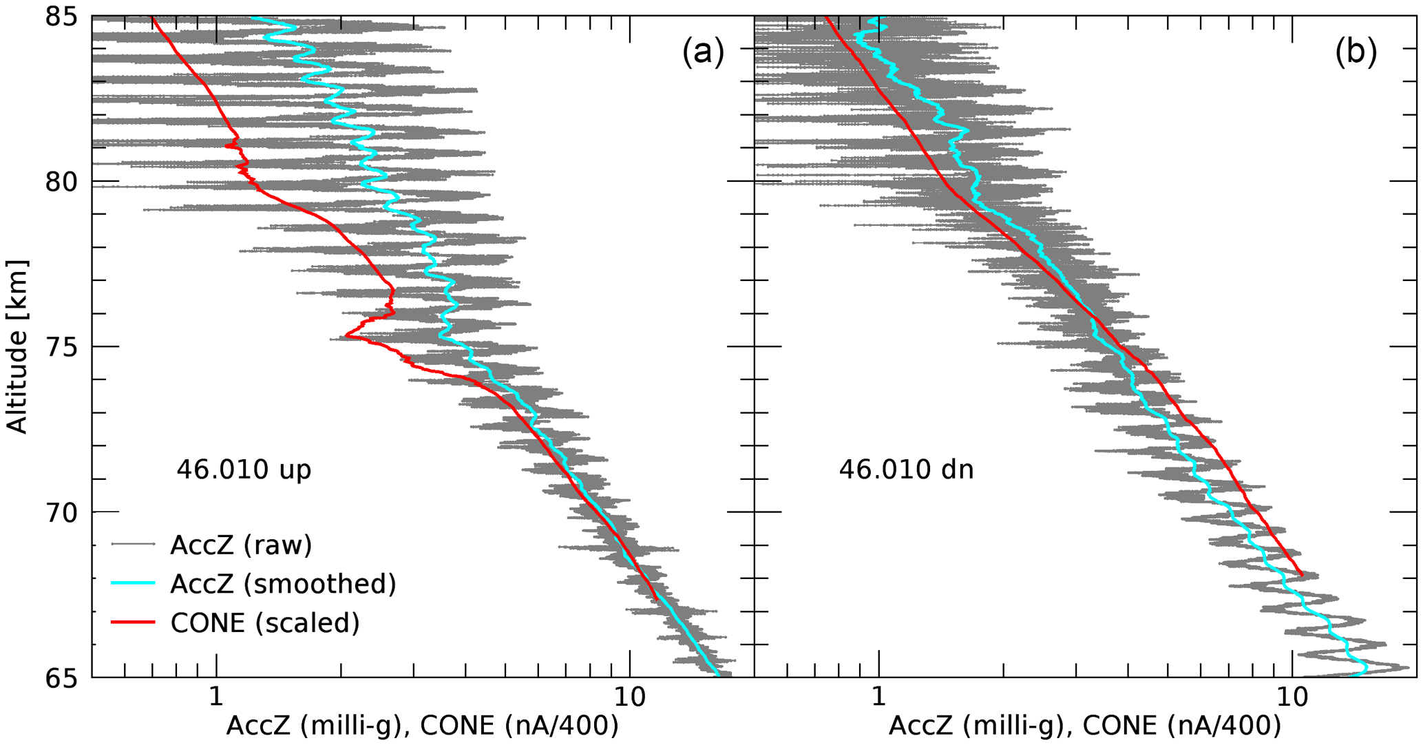
Figure A1 shows the accelerometer data (raw data in grey and smoothed data in cyan) compared with the CONE ion currents (red) for flight 46.010. First, the CONE currents are almost identical except for the major perturbations around 75 and 80 km discussed in the main text and Fig. 2. The good agreement between all four current profiles suggests that atmospheric densities are not very different for upleg and downleg in the lower mesosphere.
Next, we show the acceleration component along the z axis (payload spin axis). Please note that we have subtracted a constant bias from the accelerometer data, which was determined at altitudes above 120 km from the raw data. For both upleg and downleg, the acceleration residuals decrease exponentially with altitude. The upleg portion of flight 46.010 shows a small spin modulation (grey line), which is consistent with a larger coning half angle of 1.3∘ observed by the onboard gyroscope (as compared to 0.5∘ on downleg). On the other hand, the stable attitude on the downleg begins to deteriorate at 70 km, which is visible in the beginning spin modulation in the downleg accelerometer data. The cyan line is a running mean to reduce this spin modulation and noise. Considering these flight conditions, we suggest that the smoothed, residual accelerations can be interpreted as measure of the atmospheric drag force on the payload, which we write as
where m is the payload mass, ρ the atmospheric density, Cd the drag coefficient, A the cross-sectional area of the payload, and v the payload velocity. Since the payload velocity was aligned with the accelerometer z axis, almost all drag was registered in the z channel of the three-axis accelerometer. The x and y channels registered less than 1 mg throughout these stable portions of the flight.
A DSMC of the supersonic flow using the velocity, density, and temperature conditions for this flight yielded a drag force of 7.2 N at 75 km. We used the NASA DAC97 package for our simulations (LeBeau, 1999). Dividing the force by the payload mass of 187 kg, this corresponds to an acceleration of 4.0 mg, which is close to the observed (average) accelerations of 3.7 and 3.3 mg on upleg and downleg. This calculation and the exponential decrease of the acceleration values gives us confidence that the accelerometer signal is due to drag acceleration.
The perturbations in the CONE measurement were unexpected and unprecedented, and the simultaneous change in acceleration of 0.5 mg (especially near 75 km) can provide additional clues. No ACS maneuver or other payload event occurred at this time that could have perturbed the measurement, therefore it is suggested that a large wind may have altered the drag force. We performed DSMC simulations adding winds and found that a horizontal wind of 100 m s−1, which reduces the ram flow by 30 m s−1, can indeed reduce the drag force and the relevant acceleration component by 5 % or 0.2 mg. Additional vertical winds could add to this change. Qualitatively, it seems plausible that a strong wind could have caused a small change in the drag force, and possibly also the disturbance in the CONE ionization gauge, which is directly exposed to the flow.
While sensitive accelerometers on supersonic free-falling spheres have been used previously to successfully measure winds, densities and temperatures in the mesosphere and lower thermosphere (Philbrick et al., 1985), this experiment demonstrates that changes in atmospheric drag may be observed for much heavier, cylindrical payloads with a low-cost device, however, only in the denser mesosphere. A similar accelerometer experiment was flown on the German MAPHEUS-1 student mission (Stamminger et al., 2009), which appears less sensitive than our device. More sensitive and lower-noise accelerometers could provide a basic method for routine wind and density measurements in the mesosphere.
GAL is co-investigator of the MTeX project, performed the sounding rocket data analysis, drafted the manuscript and prepared the figures. RLC is the principal investigator of the MTeX project and provided the lidar data. AB is co-investigator of the MTeX project and provided the accelerometer experiment. MFL is the principal investigator of the MIST project and provided the tracer images and wind profiles. BS provided the ionization gauges and the code for the wavelet based turbulence analysis. All co-authors provided scientific input as a team effort and during the manuscript preparation and review process.
The authors declare that they have no conflict of interest.
This research was supported by NASA grants NNX13AE35G (Embry-Riddle
Aeronautical University), NNX13AE26G and NNX14AH45G (Clemson University), and
NNX13AE31G (University of Alaska Fairbanks). The CONE sensors were built by
Hans-Jürgen Heckl and calibrated by Arthur Szewczyk at the Institute for
Atmospheric Physics in Kühlungsborn, Germany. The CONE electronics was
designed and built by von Hoerner & Sulger GmbH, Schwetzingen, Germany. We
thank NASA Wallops Flight Facility and Poker Flat Research Range for mission
and payload design and launch and recovery operations.
The topical editor, Petr Pisoft, thanks
two anonymous referees for help in evaluating this paper.
Blamont, J. E. and de Jager, C.: Upper atmospheric turbulence near the 100 km level, Ann. Geophys., 17, 134–144, 1961. a, b
Blix, T. A., Thrane, E. V., and Andreassen, Ø.: In situ measurements of fine scale structure and turbulence in the mesosphere and lower thermosphere by means of electrostatic positive ion probes, J. Geophys. Res., 95, 5533–5548, https://doi.org/10.1029/JD095iD05p05533, 1990. a
CCMC (Community Coordinated Modeling Center): NRLMSISE-00 Atmosphere Model, Dr. Masha Kuznetsova, https://ccmc.gsfc.nasa.gov/modelweb/models/nrlmsise00.php, last access: 13 August 2018.
Collins, R. L., Lehmacher, G. A, Larsen, M. F., and Mizutani, K.: Estimates of vertical eddy diffusivity and energy dissipation in the upper mesosphere in the presence of a mesospheric inversion layer, Ann. Geophys., 29, 2019–2029, https://doi.org/10.5194/angeo-29-2019-2011, 2011. a, b
Collins R., Triplett, C., Barjatya, A., Lehmacher, G., and Fritts, D.: Using lidar and rockets to explore turbulence in the atmosphere, SPIE Newsroom, https://doi.org/10.1117/2.1201505.005922, 2015. a, b
Fritts, D. C. and Alexander, M. J.: Gravity dynamics and effects in the middle atmosphere, Rev. Geophys., 41, 1003, https://doi.org/10.1029/2001RG000106, 2003. a
Fritts, D. C., Laughman, B., Wang, L., Lund, T. S., and Collins, R. L.: Gravity Wave Dynamics in a Mesospheric Inversion Layer: 1. Reflection, Trapping, and Instability Dynamics, J. Geophys. Res., 123, 626–648, https://doi.org/10.1002/2017JD027440, 2018a. a, b
Fritts, D. C., Wang, L., Laughman, B., Lund, T. S., and Collins, R. L.: Gravity Wave Dynamics in a Mesospheric Inversion Layer: 2. Instabilities, Turbulence, Fluxes, and Mixing, J. Geophys. Res.-Atmos., 123, 649–670, https://doi.org/10.1002/2017JD027442, 2018b. a, b, c, d, e, f, g
Giebeler, J., Lübken, F.-J., and Nägele, N.: CONE – a new sensor for in situ observations of neutral and plasma density fluctuations, Proc. 11th ESA Symp. Europ. Rocket Balloon Progr., Montreux, Switzerland, ESA SP-355, 311–318, 1993. a, b
Heisenberg, W.: Zur statistischen Theorie der Turbulenz, Z. Phys., 124, 628–657, https://doi.org/10.1007/BF01668899, 1948. a
Hillert, W., Lübken, F.-J., and Lehmacher, G.: TOTAL: a rocket-borne instrument for high resolution measurements of neutral air turbulence during DYANA, J. Atmos. Terr. Phys., 56, 1835–1852, 1994. a
Howard, L. N.: Note on a paper of John W. Miles, J. Fluid Mech., 10, 509–512, 1961. a
Kolmogorov, A. N.: The local structure of turbulence in incompressible viscous fluid for very large Reynolds numbers (Russian), P. USSR Acad. Sci., 30, 299–303, 1941. a
Larsen, M. F., Christensen, A. B., and Odom, C. D.: Observations of unstable atmospheric shear layers in the lower E region in the post-midnight auroral oval, Geophys. Res. Lett., 24, 1915–1918, https://doi.org/10.1029/97GL01942, 1997. a, b
Larsen, M. F.: Winds and shears in the mesosphere and lower thermosphere: Results from four decades of chemical release wind measurements, J. Geophys. Res., 107, 1215–1229, https://doi.org/10.1029/2001JA000218, 2002. a, b
LeBeau, G. J.: A Parallel Implementation of the Direct Simulation Monte Carlo Method, Comp. Methods Appl. Mech. Eng., 174, 319–337, 1999. a
Lehmacher, G. and Lübken, F.-J.: Simultaneous observation of convective adjustment and turbulence generation in the mesosphere, Geophys. Res. Lett., 22, 2477–2480, https://doi.org/10.1029/95GL02351, 1995. a, b
Lehmacher, G. A., Croskey, C. L., Mitchell, J. D., Friedrich, M., Lübken, F.-J., Rapp, M., Kudeki, E., and Fritts, D. C.: Intense turbulence observed above a mesospheric temperature inversion at equatorial latitude, Geophys. Res. Lett., 33, L08808, https://doi.org/10.1029/2005GL024345, 2006. a, b, c
Lehmacher, G. A., Scott, T. D., Larsen, M. F., Bilén, S. G., Croskey, C. L., Mitchell, J. D., Rapp, M., Lübken, F.-J., and Collins, R. L.: The Turbopause experiment: atmospheric stability and turbulent structure spanning the turbopause altitude, Ann. Geophys., 29, 2327–2339, https://doi.org/10.5194/angeo-29-2327-2011, 2011. a, b, c, d, e, f, g, h
Liu, H.-L., Hagan, M. E., and Roble, R. G.: Local mean state changes due to gravity wave breaking modulated by the diurnal tide, J. Geophys. Res., 105, 12381–12396, https://doi.org/10.1029/1999JD901163, 2000. a, b
Lübken, F.-J. and von Zahn, U.: Thermal structure of the mesopause region at polar latitudes, J. Geophys. Res., 96, 20841–20857, 1991. a
Lübken, F.-J.: On the extraction of turbulent parameters from atmospheric density fluctuations, J. Geophys. Res., 97, 20385–20395, https://doi.org/10.1029/92JD01916, 1992. a
Lübken, F.-J.: Seasonal variation of turbulent energy dissipation rates at high latitudes as determined by in situ measurements of neutral density fluctuations, J. Geophys. Res., 102, 13441–13456, https://doi.org/10.1029/97JD00853, 1997. a, b, c, d
Lübken, F.-J., Hillert, W., Lehmacher, G., and von Zahn, U.: Experiments revealing small impact of turbulence on the energy budget of the mesosphere and thermosphere, J. Geophys. Res., 98, 20369–20384, https://doi.org/10.1029/93JD02055, 1993. a, b, c, d, e, f, g
Meraner, K. and Schmidt, H.: Transport of nitrogen oxides through the winter mesopause in HAMMONIA, J. Geophys. Res.-Atmos., 121, 2556–2570, https://doi.org/10.1002/2015JD024136, 2016. a
Meriwether, J. W. and Gerrard, A. J.: Mesosphere inversion layers and stratosphere temperature enhancements, Rev. Geophys., 42, RG3003, https://doi.org/10.1029/2003RG000133, 2004. a, b
Miles, J. W.: On the stability of heterogeneous shear flows, J. Fluid Mech., 10, 496–512, 1961. a
Offermann, D., Gusev, O., Donner, M, Forbes, J. M., Hagan, M., Mlynczak, M. G., Oberheide, J., Preusse, P., Schmidt, H., and Russell III, J. M.: Relative intensities of middle atmosphere waves, J. Geophys. Res., 114, D06110, https://doi.org/10.1029/2008JD010662, 2009. a
Philbrick, C. R., Schmidlin, F. J., Grossmann, K. U., Lange, G., Offermann, D., Baker, K. D., Krankowsky, D., and von Zahn, U.: Density and temperature structure over northern Europe, J. Atmos. Terr. Phys., 47, 159–172, https://doi.org/10.1016/0021-9169(85)90131-X, 1985. a
Picone, J. M., Hedin, A. E., Drob, D. P., and Aikin, A. C.: NRLMSISE-00 empirical model of the atmosphere: Statistical comparisons and scientific issues, J. Geophys. Res., 107, 1468, https://doi.org/10.1029/2002JA009430, 2002. a
Qian, L., Solomon, S. C., and Kane, T. J.: Seasonal variation of thermospheric density and composition, J. Geophys. Res., 114, A01312, https://doi.org/10.1029/2008JA013643, 2009. a
Rapp, M., Gumbel, J., and Lübken, F.-J.: Absolute density measurements in the middle atmosphere, Ann. Geophys., 19, 571–580, https://doi.org/10.5194/angeo-19-571-2001, 2001. a, b, c, d, e, f, g, h, i
Roberts, B. C. and Larsen, M. F.: Structure function analysis of chemical tracer trails in the mesosphere-lower thermosphere region, J. Geophys. Res.-Atmos., 119, 6368–6375, https://doi.org/10.1002/2013JD020796, 2014. a, b, c, d
SABER: SABER Sounding of the Atmosphere using Broadband Emission Radiometry, GATS Team, Tolvey G. Bird, Data Management and Computer Systems, http://saber.gats-usa.net/index.php, last access: 13 August 2018.
Snively, J. B.: Nonlinear gravity wave forcing as a source of acoustic waves in the mesosphere, thermosphere, and ionosphere, Geophys. Res. Lett., 44, 12020–12027, https://doi.org/10.1002/2017GL075360, 2017. a
Stamminger, A., Ettl, J., Blochberger, G., Drescher, J., Griesche, A., Hassenpflug, F., Hoepfner, S., Hörschgen, M., Meyer, A., Neumann, C., Ratke, L., Plescher, E., and Willnecker, R.: MAPHEUS-1: Vehicle, subsystem design, flight performance and experiments, Proc. 19th ESA Symp. Europ. Rocket Balloon Progr., Bad Reichenhall, Germany, ESA SP-671, 2009. a
Strelnikov, B., Rapp, M., and Lübken, F.-J.: A new technique for the analysis of neutral air density fluctuations measured in situ in the middle atmosphere, Geophys. Res. Lett., 30, 2052, https://doi.org/10.1029/2003GL018271, 2003. a, b, c, d
Strelnikov, B., Rapp, M., and Lübken, F.-J.: In situ density measurements in the mesosphere/lower thermosphere region with the TOTAL and CONE instruments, in: An Introduction to Space Instrumentation, edited by: Oyama, K. and Cheng, C. Z., Terrapub, https://doi.org/10.5047/aisi.001, 1–11, 2013. a
Strelnikov, B., Szewczyk, A., Strelnikova, I., Latteck, R., Baumgarten, G., Lübken, F.-J., Rapp, M., Fasoulas, S., Löhle, S., Eberhart, M., Hoppe, U.-P., Dunker, T., Friedrich, M., Hedin, J., Khaplanov, M., Gumbel, J., and Barjatya, A.: Spatial and temporal variability in MLT turbulence inferred from in situ and ground-based observations during the WADIS-1 sounding rocket campaign, Ann. Geophys., 35, 547–565, https://doi.org/10.5194/angeo-35-547-2017, 2017. a, b, c
Szewczyk, A.: Mesospheric Turbulence: The Role in the Creation of Mesospheric Inversion Layers and Statistical Results, Ph. D. thesis, University of Rostock, Germany, 148 pp., available at: http://rosdok.uni-rostock.de/site/epub (last access: 13 August 2018), 2015. a, b, c, d
Szewczyk, A., Strelnikov, B., Rapp, M., Strelnikova, I., Baumgarten, G., Kaifler, N., Dunker, T., and Hoppe, U.-P.: Simultaneous observations of a mesospheric inversion layer and turbulence during the ECOMA-2010 rocket campaign, Ann. Geophys., 31, 775–785, https://doi.org/10.5194/angeo-31-775-2013, 2013. a, b
Torrence, C. and Compo, G. P.: A practical guide to wavelet analysis, Bull. Am. Meteorol. Soc., 79, 61–78, https://doi.org/10.1175/1520-0477, 1998. a
Triplett, C. C., Li, J., Collins, R. L., Lehmacher, G. A., Barjatya, A., Fritts, D. C., Strelnikov, B., Lübken, F.-J., Thurairajah, B., Harvey, V. L., Hampton, D. L., and Varney, R. H.: Observations of reduced turbulence and wave activity in the Arctic middle atmosphere following the January 2015 stratospheric sudden warming, J. Geophys. Res.-Atmos., in review, 2018. a, b, c, d, e, f, g, h, i
Xu, J., Smith, A. K., Collins, R. L., and She, C.-Y.: Signature of an overturning gravity wave in the mesospheric sodium layer: Comparison of a nonlinear photochemical-dynamical model and lidar observations, J. Geophys. Res., 111, D17301, https://doi.org/10.1029/2005JD006749, 2006. a, b